Bag of Words (BoW) & TF-IDF

A bag of words throws away everything the last two phases were about. No order, no context, no sequence — just how often each word appears. It should be hopeless.

On 8,000 IMDB reviews it scores 0.8748, which is better than every recurrent model measured in Phase 4 — a GRU reached 0.8156 there — and it trains in 0.4 seconds.

That is the baseline every neural model on the following pages has to beat, and this page is about making it as strong as it deserves to be.

What you’ll learn

The document-term matrix, and why it is stored sparse: 0.0046 density at 30,000 features, 13.2 MB against 1,920 MB dense.
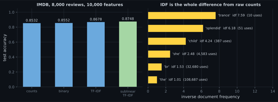
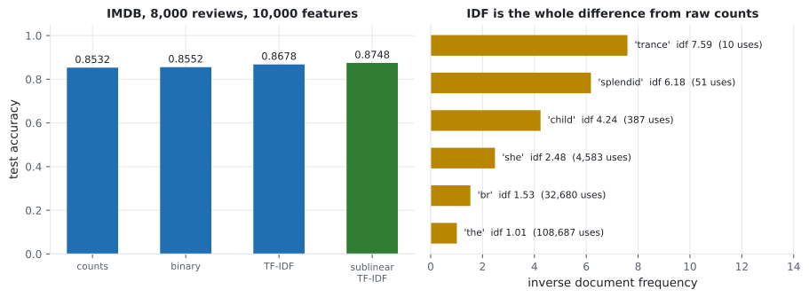
Four weightings measured: counts 0.8532, binary 0.8552, TF-IDF 0.8678, sublinear TF-IDF 0.8748.
What IDF actually does to a word’s weight, from the (1.008) to trance (7.589).
Why TF-IDF at 2,000 features beats raw counts at 30,000.
Why sublinear TF-IDF also converged 21× faster than raw counts.
What the fitted weights tell you — a linear model over words is readable in a way no model in this module is.

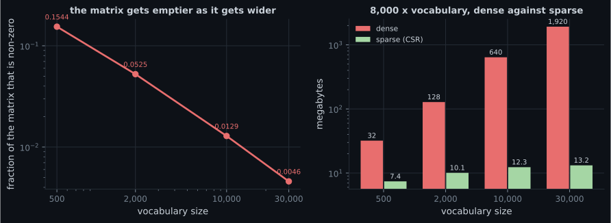
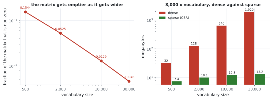
The document-term matrix

Each row is a document, each column a vocabulary word, each entry a count.

X_{ij} = \text{count of word } j \text{ in document } i

The matrix is enormous and almost entirely zeros, because any one review uses a tiny slice of the vocabulary.

Vocabulary	Non-zeros per document	Density	Sparse (CSR)	Dense
500	77.2	0.1544	7.4 MB	32 MB
2,000	104.9	0.0525	10.1 MB	128 MB
10,000	128.6	0.0129	12.3 MB	640 MB
30,000	137.4	0.0046	13.2 MB	1,920 MB

Two panels. Left: density against vocabulary size on log axes, falling from 0.1544 at 500 features to 0.0046 at 30,000. Right: bars of memory on a log scale comparing dense storage rising from 32 MB to 1,920 MB against sparse CSR storage rising only from 7.4 MB to 13.2 MB. — Going from 500 to 30,000 features multiplies the dense matrix by 60 and the sparse one by 1.8, because a review only gains 60 more non-zero entries — from 77 words to 137. That gap is why every text pipeline uses `scipy.sparse` and why `.toarray()` on a document-term matrix is the classic way to exhaust a machine's memory.

The four weightings

The scheme is not a detail. It was worth more than a 15× larger vocabulary here.

Scheme	Formula	Accuracy	Seconds to fit
raw counts	$c_{ij}$	0.8532	8.5
binary	$\mathbb{1}[c_{ij} > 0]$	0.8552	2.9
TF-IDF	$c_{ij}\cdot\log\frac{N}{1+n_j}$	0.8678	0.7
sublinear TF-IDF	$(1 + \log c_{ij})\cdot\text{idf}_j$	0.8748	0.4

Two panels. Left: bars of test accuracy for counts 0.8532, binary 0.8552, TF-IDF 0.8678 and sublinear TF-IDF 0.8748. Right: horizontal bars of inverse document frequency for six words, from 'the' at 1.01 with 108,687 uses up to 'trance' at 7.59 with 10 uses. — The weighting is worth +0.0216 from the worst to the best scheme — and the fit time falls from 8.5 seconds to 0.4. Raw counts give a badly conditioned problem: one feature ('the') has values in the hundreds while most have values of 0 or 1, so the optimiser crawls. Scaling by IDF and compressing counts with a logarithm fixes the conditioning as much as it fixes the statistics.

What IDF does

\text{idf}_j = \log\frac{N}{1 + n_j} + 1

where $n_j$ is the number of documents containing word $j$ . Measured on this corpus:

Rank	Word	Uses	IDF
1	`the`	108,687	1.008
6	`br`	32,680	1.532
51	`she`	4,583	2.480
501	`child`	387	4.238
3,001	`splendid`	51	6.181
10,000	`trance`	10	7.589

IDF is a smooth, learned-from-data version of a stopword list. the appears in nearly every document, so it gets a weight of ~1 and its count — the largest number in the matrix — stops dominating. Nothing was hand-listed, and nothing was deleted; the previous page’s stopword removal threw away 32.7% of the corpus to achieve less.

Note br at 1.532: the HTML remnant is common enough to be down-weighted automatically.

Why sublinear TF helps

A review that says “terrible” eight times is not eight times more negative than one that says it once. $1 + \log c$ encodes that: the second occurrence adds 0.69, the eighth adds 0.13. It was worth +0.0070 here — the largest single gain in the table.

Vocabulary size matters less than weighting

Features	Counts	TF-IDF
500	0.8265	0.8290
2,000	0.8353	0.8625
10,000	0.8532	0.8678
30,000	0.8592	0.8658

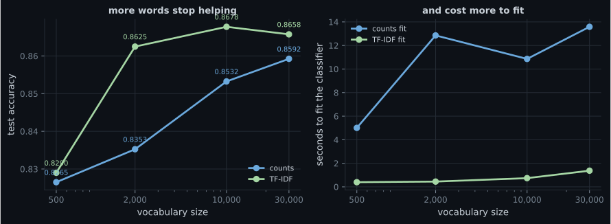
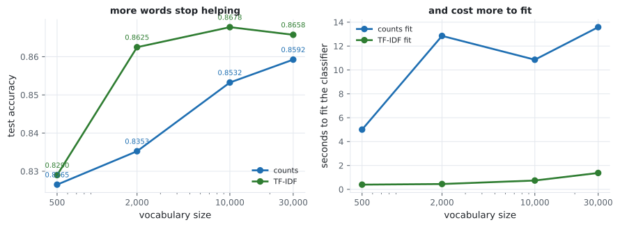
Two panels. Left: test accuracy against vocabulary size for counts and TF-IDF, with TF-IDF above counts at every size and peaking at 10,000 features before dipping at 30,000. Right: seconds to fit the classifier against vocabulary size, rising steeply for counts and staying low for TF-IDF. — Two things to read here. TF-IDF at 2,000 features (0.8625) beats raw counts at 30,000 (0.8592): the weighting is worth more than a fifteen-fold larger vocabulary. And TF-IDF peaks at 10,000 and then declines slightly — the words between rank 10,000 and 30,000 appear in a handful of documents each, so they mostly let the model memorise.

The rank-10,000 word appears 10 times in 8,000 reviews. A feature that fires on one document in eight hundred cannot generalise; it can only memorise. This is the same once-seen tail measured on the preprocessing page, now visible as a dip in accuracy.

The part no neural model gives you

What the model learned, in words

weights = model.coef_[0]
order = np.argsort(weights)
print("negative:", [names[i] for i in order[:10]])
print("positive:", [names[i] for i in order[-10:]])

text

negative: worst, bad, awful, waste, nothing, terrible, poor, script, no, boring
positive: amazing, favorite, love, perfect, wonderful, and, well, best, excellent, great

Those two lines are the entire model, and they are checkable by a human being. script in the negative list is a nice detail — people mention the script when it is bad — and and in the positive list is a reminder that a linear model will happily use a function word as a weak sentiment cue if the correlation exists.

Compare that with the Grad-CAM page, where extracting a much vaguer explanation from a convnet took gradient tapes, a sanity check against random weights, and 441 forward passes for occlusion.

diagram Diagram mermaid

  flowchart LR
  A["documents"] --> B["CountVectorizer
max_features"]
  B --> C["sparse matrix
0.0046 density"]
  C --> D{"weighting"}
  D -->|"counts"| E["0.8532, 8.5s"]
  D -->|"binary"| F["0.8552, 2.9s"]
  D -->|"tf-idf"| G["0.8678, 0.7s"]
  D -->|"sublinear tf-idf"| H["0.8748, 0.4s"]
  H --> I["LogisticRegression
readable weights"]

What a bag of words cannot do

It scored 0.8748 without knowing what order the words came in. Everything it cannot do follows from that:

Phrase	What the model sees	Problem
“not good” vs “good”	`not`, `good` vs `good`	negation is a separate feature, not a modifier
“the film was bad, the acting good”	all four words	no idea which noun each adjective attaches to
“unpredictable plot” vs “unpredictable service”	same words, different sentiment	no context

The standard patch is n-grams — treat not good as one feature — which works and explodes the vocabulary: bigrams on this corpus would be roughly 40× the columns. Sequence models exist because that patch does not scale, and the honest measurement is that on this task the patch is barely needed.

sketch TF, IDF and the product p5.js

Drag a word's document frequency and see how IDF re-weights it. The measured corpus values are marked.

sketch The measured table, ranked p5.js

Click a column to rank every row by it. The bars are that column's values and the highest and lowest are computed from the numbers, not written in.

Pitfalls

Calling .toarray() on a document-term matrix. 1,920 MB dense against 13.2 MB sparse at 30,000 features.
Using raw counts. 0.8532 against 0.8748, and 8.5 seconds to fit against 0.4 — badly scaled features are slow as well as worse.
Fitting the vectorizer on train and test. The IDF weights are learned parameters; fitting them on the test set leaks document frequencies.
Reaching for a bigger vocabulary before a better weighting. TF-IDF at 2,000 features beat counts at 30,000.
Assuming more features always help. TF-IDF peaked at 10,000 and fell at 30,000, where the added words appear ten times in the whole corpus.
Skipping this baseline before training a sequence model. It scored 0.8748 in 0.4 seconds; a GRU in Phase 4 managed 0.8156 in 52.3.
Trusting the top-weight list as a causal explanation. and sits in the positive list — a correlation the model exploits, not a fact about English.

Recap

A document-term matrix is 0.0046 dense at 30,000 features; sparse storage is 13.2 MB against 1,920 MB.
Weightings on 8,000 IMDB reviews: counts 0.8532, binary 0.8552, TF-IDF 0.8678, sublinear TF-IDF 0.8748.
Sublinear TF-IDF also fit 21× faster than raw counts (0.4 s against 8.5 s).
IDF ranged from 1.008 (the) to 7.589 (trance) — a data-driven stopword list that deletes nothing.
TF-IDF at 2,000 features (0.8625) beat counts at 30,000 (0.8592); TF-IDF peaked at 10,000.
The fitted weights are directly readable: worst, bad, awful… against amazing, favorite, love….

Bag of words treats good and great as unrelated columns. Embeddings fix that, and the next page measures what it is worth: Word Embeddings (Word2Vec, GloVe).

pch.quizTag pch.quizDefaultTitle

Sublinear TF-IDF scored 0.8748 while raw counts scored 0.8532 — and fit in 0.4 seconds against 8.5. Why is the weighting worth so much?

pch.quizShowAnswer

B — Raw counts are badly conditioned: 'the' takes values in the hundreds while most features are 0 or 1, so one column dominates and the optimiser crawls. IDF and the log both fix the scale — Both the accuracy and the twenty-one-fold speed-up come from the same cause, which is why the scheme is not a cosmetic choice.
A 30,000-feature document-term matrix over 8,000 reviews is 0.0046 dense. What does that mean in practice?

pch.quizShowAnswer

B — Dense storage would be 1,920 MB against 13.2 MB sparse — calling .toarray() on it is the classic way to exhaust a machine's memory — A review contains about 137 distinct words out of 30,000 columns, and that ratio only gets worse as the vocabulary grows.
TF-IDF at 2,000 features scored 0.8625; raw counts at 30,000 scored 0.8592. What is the lesson?

pch.quizShowAnswer

B — Fix the weighting before enlarging the vocabulary — the scheme was worth more than a fifteen-fold increase in features — TF-IDF also peaked at 10,000 and dipped at 30,000, because the rank-10,000 word appears just ten times in the whole corpus.
IDF gave 'the' a weight of 1.008 and 'trance' 7.589. How does that relate to stopword removal?

pch.quizShowAnswer

B — It is a smooth, data-driven version of the same idea — common words are flattened towards 1 rather than deleted, so no information is thrown away — The preprocessing page's stopword list deleted 32.7% of all tokens to achieve less. IDF also caught 'br', the HTML remnant, without anyone listing it.
A bag of words scored 0.8748 while a GRU in Phase 4 scored 0.8156. What follows?

pch.quizShowAnswer

B — This baseline must be measured before any sequence model is claimed to work — on a task decidable from word presence, order buys little, and the neural model has to earn its cost — The two runs used different corpus sizes, so it is not a controlled comparison — but that is the point: without running this baseline you cannot tell whether your sequence model is doing anything.

🧪 Try It Yourself

pch.coffeeTagline

pch.coffeeCta

pch.feedbackHeading

pch.feedbackSubheading