Text Preprocessing (Tokenization, Stemming, Lemmatization)

A network takes numbers. Text is not numbers, and every decision on the way from one to the other — where a token starts, what counts as the same word, which words to keep — is made before the model sees anything and cannot be undone by training.

This page counts those decisions on 5,000 IMDB reviews decoded back into words: 1,219,106 tokens, 43,783 distinct ones. It opens with an uncomfortable observation about that corpus, because it is the most common way this material misleads people.

The decisions were already made for you

keras.datasets.imdb ships integer ids, not text. Somebody already tokenized, lowercased and stripped punctuation. Apply those steps yourself and watch nothing happen:

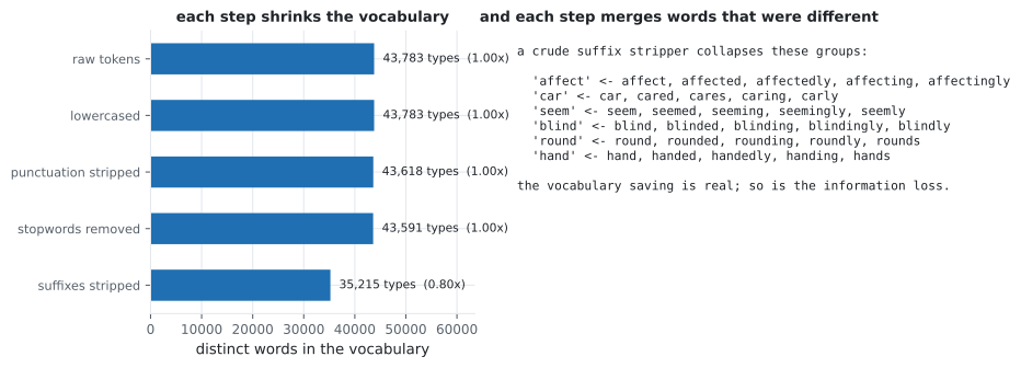
Step	Distinct words	Tokens
raw (as shipped)	43,783	1,219,106
lowercased	43,783	1,219,106
punctuation stripped	43,618	1,218,706
27 stopwords removed	43,591	820,241
suffixes stripped	35,215	820,241

Lowercasing changes the vocabulary by zero words. Stripping punctuation removes 165. If you benchmark preprocessing on this dataset you will conclude that preprocessing does not matter, and you will be measuring the previous engineer’s work rather than your own.

The evidence that the cleanup was imperfect sits at rank 7 of the frequency table:

Rank	Token	Uses	Share of all tokens
1	the	68,738	0.0564
2	and	33,462	0.0274
3	a	33,325	0.0273
…
7	br	20,864	0.0171

br is the remains of <br /> tags. It is the seventh most common “word” in the corpus — ahead of in, it and i — and it carries no meaning at all. Every model in this phase spends capacity on it.

What you’ll learn

• Why the vocabulary never stops growing: Heaps’ exponent 0.573 on this corpus.
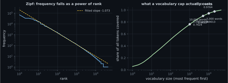
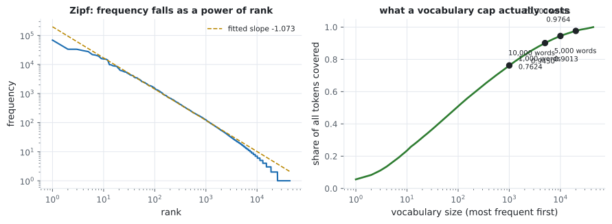
• Zipf’s law, measured: slope −1.0731 over the first 2,000 ranks.
• What a vocabulary cap costs: 10,000 words cover 0.9450 of tokens, so 5.5% of the text becomes <oov>.
• Why 42.9% of the vocabulary is words seen exactly once, and they are 1.54% of the text.
• What each normalisation step buys and what it destroys.
• Where classic preprocessing ends and subword tokenization begins.

The two laws that shape every vocabulary

figure 5,000 IMDB reviews matplotlib

The left curve is Heaps' law: distinct words grow as tokens^0.573, so reading twice as much text still turns up about 49% more new words. It never saturates, which is why 'just use the whole vocabulary' is not a strategy. The right panel says what those extra words are — 42.9% of the vocabulary appeared exactly once, and no model learns anything from a single occurrence.

$$V(n) = k\,n^{\beta}, \quad \beta = 0.573 \qquad\qquad f(r) \propto r^{-s}, \quad s = 1.0731$$

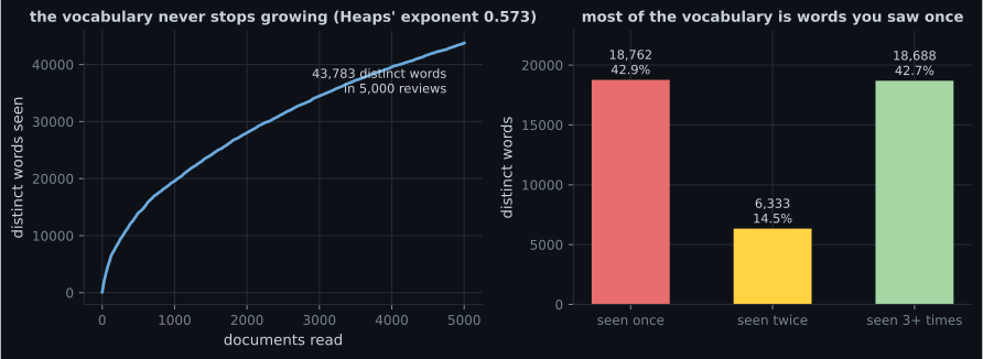
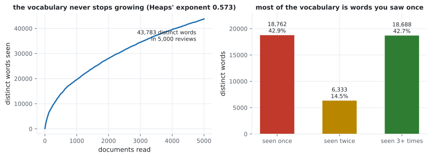
Heaps’ law says the vocabulary grows without bound. Zipf’s law says the extra words are nearly worthless: frequency falls as roughly $1/r$, so a few thousand words are almost all of the text.

figure Zipf's law and what it means for a vocabulary cap matplotlib

The straight line on log-log axes is the law. The right panel is the practical consequence, and the reason 10,000 is such a common default: it covers 94.5% of tokens with a quarter of the words. The flat tail on the left — the step down to frequency 1 — is those 18,762 once-seen words, and it is also why the slope is fitted over the first 2,000 ranks only.

Vocabulary	Token coverage	OOV rate
1,000	0.7624	0.2376
5,000	0.9013	0.0987
10,000	0.9450	0.0550
20,000	0.9764	0.0236

Every OOV rate there is text your model never sees. Doubling the vocabulary from 10,000 to 20,000 halves the loss — and doubles the embedding matrix. The next page gets the OOV rate to exactly zero without either cost.

Normalisation: what it buys, what it destroys

figure Each step shrinks the vocabulary — and merges words that were different matplotlib

Only the last step does real work on this corpus, cutting the vocabulary by 19.6%. The right panel is the price: 'affectingly' and 'affects' become one token, and so do 'car' and 'caring' — a collision no dictionary-based lemmatizer would make. Removing 27 stopwords left the vocabulary almost unchanged (43,618 to 43,591) while deleting 32.7% of all tokens, which is exactly what stopwords are: a handful of types carrying enormous mass.

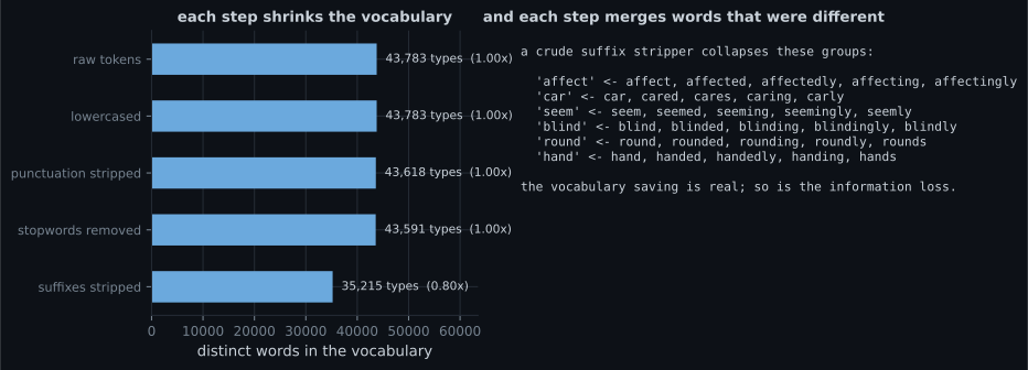
Technique	What it does	Cost
lowercasing	The → the	loses US vs us, Apple vs apple
punctuation stripping	don't → dont	splits or merges contractions inconsistently
stopword removal	drops the, a, of…	32.7% of tokens gone; destroys negation and phrasing
stemming	affecting → affect	rule-based; merges words that differ
lemmatization	better → good	dictionary-based, slower, needs a POS tagger

Two of these deserve a warning rather than a description:

• Stopword removal deleted 32.7% of the corpus. For a bag-of-words model that is usually harmless. For anything that reads word order it is destructive — “not good” and “good” become identical once not is dropped, and plenty of published stopword lists contain not.
• Stemming merges words a reader would not. The measured collisions include car, cared, cares, caring → car. It buys a 19.6% smaller vocabulary; whether that is worth it depends on whether your model has enough data to learn the inflections separately.

Modern practice is to do less of this, not more. Subword tokenization removes the vocabulary pressure that made aggressive normalisation attractive, and a model with enough data learns that “affects” and “affecting” are related without being told.

diagram Diagram mermaid

  flowchart TB
  A["raw text"] --> B["tokenize
where does a token start?"]
  B --> C{"normalise?"}
  C -->|"lowercase"| D["0 words here
already lowercase"]
  C -->|"strip punctuation"| E["-165 words"]
  C -->|"drop stopwords"| F["-32.7% of tokens"]
  C -->|"stem"| G["-19.6% of vocabulary
plus collisions"]
  D --> H["cap the vocabulary"]
  E --> H
  F --> H
  G --> H
  H --> I["10,000 words
= 5.5% OOV"]
  H --> J["subword pieces
= 0% OOV"]

sketch Zipf, coverage and the cap you choose p5.js Pause Restart

Drag the vocabulary cap. The bars follow the measured Zipf slope; the readout is what that cap covers and what it throws away.

sketch The measured table, ranked p5.js Pause Restart

Click a column to rank every row by it. The bars are that column's values and the highest and lowest are computed from the numbers, not written in.

Pitfalls

• Benchmarking preprocessing on a pre-processed corpus. Lowercasing IMDB changes the vocabulary by 0 words; you are measuring somebody else’s pipeline.
• Trusting the cleanup. br is the 7th most frequent token here, at 20,864 uses.
• Removing stopwords before a sequence model. It deleted 32.7% of tokens, and many stopword lists include not.
• Calling a rule-based suffix stripper a lemmatizer. caring → car is a measured collision, not a hypothetical one.
• Choosing a vocabulary cap without measuring coverage. 1,000 words sounds reasonable and discards 23.8% of the text.
• Assuming a bigger vocabulary is free. It is a bigger embedding matrix, and 42.9% of the words it adds appear exactly once.
• Fitting the vocabulary on train and test. The cap is learned from training data only, exactly like a scaler.

Recap

• 5,000 IMDB reviews decode to 1,219,106 tokens and 43,783 distinct words; the shipped index has 88,584 entries.
• Heaps’ law with exponent 0.573 — the vocabulary never stops growing.
• Zipf’s law with slope −1.0731 — 10,000 words cover 0.9450 of tokens, 1,000 cover 0.7624.
• 18,762 words (42.9% of the vocabulary) appear exactly once and make up 1.54% of the text.
• Lowercasing this corpus changed nothing; stopword removal deleted 32.7% of tokens; suffix stripping cut the vocabulary 19.6% and merged car with caring.
• br, an HTML remnant, is the 7th most common token.

Next

Classic preprocessing manages the vocabulary. Subword tokenization removes the problem instead, and it is what every modern model actually uses: Subword Tokenization (BPE and WordPiece).

pch.quizTag pch.quizDefaultTitle

1. Lowercasing the decoded IMDB corpus changed the vocabulary from 43,783 words to 43,783 words. What does that tell you?

   A Lowercasing never helps B This corpus was already lowercased before it shipped — benchmarking preprocessing on it measures the previous engineer's pipeline, not yours C The measurement is wrong D IMDB reviews contain no capital letters
   pch.quizShowAnswer

   B — This corpus was already lowercased before it shipped — benchmarking preprocessing on it measures the previous engineer's pipeline, not yours — keras.datasets.imdb ships integer ids. Tokenization, lowercasing and punctuation stripping all happened before you loaded it — imperfectly, since 'br' survived as the 7th most frequent token.

2. A vocabulary of 10,000 words covers 0.9450 of tokens on this corpus. What happens to the rest?

   A They are dropped from the documents entirely B They collapse to a single <oov> id — 5.5% of every review becomes one meaningless token, and no amount of training recovers it C They are split into characters D They are mapped to their nearest neighbour in the vocabulary
   pch.quizShowAnswer

   B — They collapse to a single <oov> id — 5.5% of every review becomes one meaningless token, and no amount of training recovers it — This is exactly the failure subword tokenization removes: any word can be built from a small set of pieces, so the OOV rate is zero.

3. 42.9% of the vocabulary appears exactly once, but those words are only 1.54% of the tokens. What follows for the embedding matrix?

   A Those words should get larger embeddings B Their embedding rows receive one gradient update each in the entire corpus — they cost memory and learn essentially nothing C They should be duplicated to balance the data D Nothing; embeddings handle rare words automatically
   pch.quizShowAnswer

   B — Their embedding rows receive one gradient update each in the entire corpus — they cost memory and learn essentially nothing — Heaps' law guarantees it gets worse with scale: the vocabulary grows as tokens^0.573, so more text brings proportionally more once-seen words.

4. Removing 27 stopwords deleted 32.7% of all tokens but only 27 distinct words. When is that a bad trade?

   A Whenever the corpus is large B Whenever word order matters — 'not good' becomes 'good' if 'not' is on the list, and many published lists include it C Only for languages other than English D Never; stopword removal is always safe
   pch.quizShowAnswer

   B — Whenever word order matters — 'not good' becomes 'good' if 'not' is on the list, and many published lists include it — For bag-of-words it is usually harmless. For a sequence model it destroys exactly the structure the model exists to read.

5. A crude suffix stripper merged 'car', 'cared', 'cares' and 'caring' into 'car'. What is the honest summary of stemming?

   A It is a strictly better version of lemmatization B It trades vocabulary size for precision — 19.6% fewer words here, at the cost of collisions a dictionary-based lemmatizer would not make C It is required before any neural model D It has no effect on model accuracy
   pch.quizShowAnswer

   B — It trades vocabulary size for precision — 19.6% fewer words here, at the cost of collisions a dictionary-based lemmatizer would not make — Modern practice is less normalisation, not more: subword tokenization removes the vocabulary pressure that made stemming attractive.

🧪 Try It Yourself

pch.exerciseTag pch.exerciseTitle

pch.exerciseTag pch.exerciseTitle

pch.exerciseTag pch.exerciseTitle

pch.exerciseTag pch.exerciseTitle

pch.exerciseTag pch.exerciseTitle