Famous CNN Architectures (LeNet to ResNet)

Every architecture below is famous for one idea. This page rebuilds six of those ideas in miniature, trains them on the same 6,000 Fashion-MNIST rows with the same budget, and reports what each one actually bought — which is not always what the original paper’s headline suggests, because the headline was earned at a scale a CPU cannot reach.

Read the numbers as what these ideas do at toy scale, not as a reproduction of ImageNet results. That gap is itself one of the lessons.

What you’ll learn

• The ideas in order: LeNet’s stack, AlexNet’s scale, VGG’s 3×3 discipline, Inception’s parallel branches, ResNet’s shortcut, Xception’s separable convolutions, SENet’s channel gate.
• Six miniatures measured, where VGG-ish won at 0.8800 and Xception-ish reached 0.5773 with 4,714 parameters — 99% smaller.
• Residual connections at 4 and 12 convolutions: +0.0260 from depth against plain’s +0.0033, but plain still finished ahead overall.
• Why that is the expected result at this depth, and what it takes for ResNet’s claim to show up.
• Depthwise-separable convolution counted exactly: 5.6× to 8.8× fewer parameters.
• A real bug this page hit first: BN’s moving statistics made every validation score meaningless until the momentum was lowered.

The line of descent

diagram Diagram mermaid

  flowchart LR
  A["LeNet-5 1998
conv + pool + dense"] --> B["AlexNet 2012
deeper, relu, dropout"]
  B --> C["VGG 2014
only 3x3, stacked"]
  B --> D["Inception 2014
parallel kernel sizes"]
  C --> E["ResNet 2015
identity shortcuts"]
  D --> F["Xception 2016
separable convolutions"]
  E --> G["SENet 2017
learned channel gate"]
  F --> G

Each step solved the problem the previous one created. LeNet showed the pattern worked; AlexNet showed scale mattered; VGG showed uniform small kernels beat hand-tuned ones; Inception attacked the cost of that uniformity; ResNet made depth trainable; Xception and SENet attacked cost and channel weighting.

LeNet-5 (1998)

Two convolution-and-pooling blocks then a small dense head. It established the template every later network kept: alternate feature extraction with downsampling, then classify.

AlexNet (2012)

The same shape, eight layers deep, with ReLU instead of tanh, dropout, and enough GPU memory to matter. Its contribution was not an idea but a demonstration — that depth plus data plus compute beat every hand-designed feature pipeline.

VGG (2014)

One rule: every convolution is 3×3, every pool is 2×2, and the channel count doubles at each stage. The receptive-field arithmetic justifies it — two 3×3 layers cover a 5×5 window with 18 weights per channel pair instead of 25, with an extra nonlinearity.

Inception / GoogLeNet (2014)

Rather than choosing a kernel size, run 1×1, 3×3, 5×5 and pooling in parallel and concatenate. The 1×1 convolutions before the expensive branches cut the channel count first, which is where the parameter saving comes from.

ResNet (2015)

$$\mathbf{y} = \mathcal{F}(\mathbf{x}) + \mathbf{x}$$

The block learns a residual — what to add to its input, rather than the output itself. If the best thing a block can do is nothing, it can output zero, which is easy. The gradient also reaches earlier layers through the shortcut without passing through the weights, which is what let 152-layer networks train.

The ordering matters more than it looks

shortcut = x
y = Conv2D(32, 3, padding="same", use_bias=False)(x)
y = BatchNormalization()(y)
y = Activation("relu")(y)
y = Conv2D(32, 3, padding="same", use_bias=False)(y)
y = BatchNormalization()(y)
x = Add()([y, shortcut])
x = Activation("relu")(x)          # after the merge, not before

Putting the ReLU before the add and none after is a real trap, and it is the first thing I got wrong building this page: the block then adds non-negative values at every depth, activations grow without bound, and the deeper network gets worse — which looks like evidence against residual connections and is actually a bug.

Xception (2016)

Replace each convolution with a depthwise pass (one filter per input channel) followed by a pointwise 1×1 mixing step:

$$\underbrace{k^2 c_{\text{in}} c_{\text{out}}}_{\text{standard}} \quad\longrightarrow\quad \underbrace{k^2 c_{\text{in}}}_{\text{depthwise}} + \underbrace{c_{\text{in}} c_{\text{out}}}_{\text{pointwise}}$$

figure Depthwise-separable convolution, counted exactly matplotlib

At 16 channels a separable layer saves 5.6x; at 512 it saves 8.8x. The saving grows with channel count because the standard layer's cost is quadratic in channels while the depthwise part is linear. The ceiling is the kernel area — 3x3 = 9 — which is why the ratio approaches but never reaches 9.

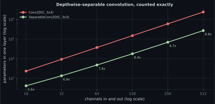
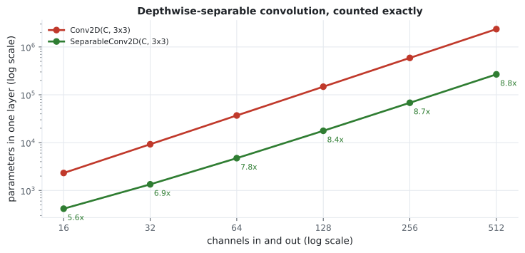
Channels in and out	Standard 3×3	Separable 3×3	Ratio
16	2,320	416	5.6×
64	36,928	4,736	7.8×
256	590,080	68,096	8.7×
512	2,359,808	267,264	8.8×

SENet (2017)

Squeeze each channel to one number with global pooling, pass those through a tiny two-layer network, and use the sigmoid output to rescale each channel. It is a learned answer to “which feature maps matter for this image”, and it costs almost nothing.

Six miniatures, one dataset

Each model below is a small version of one idea, trained identically: 6,000 Fashion-MNIST rows, 8 epochs, Adam at 1e-3, same seed.

figure Miniature versions of six ideas, same data and budget matplotlib

Accuracy tracks parameter count on this problem more than it tracks cleverness: VGG-ish has 99 times Xception-ish's parameters and 0.30 more accuracy. Inception-ish is the slowest at 306.7 seconds — its parallel 5x5 branch runs at full resolution — while returning 0.6913. None of these is a fair reproduction; they are the same ideas at 1/1000 of the scale that made them famous.

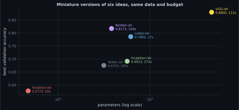
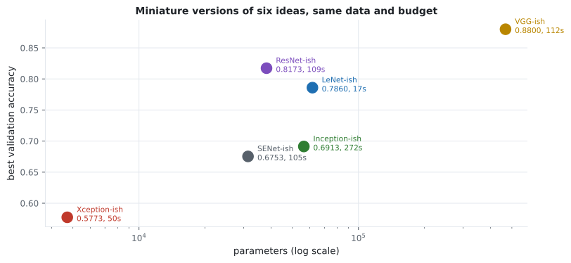
Miniature	Parameters	Best val accuracy	Seconds
LeNet-ish	61,706	0.7860	20.6
VGG-ish	467,818	0.8800	128.8
Inception-ish	56,394	0.6913	306.7
ResNet-ish	38,122	0.8173	129.1
Xception-ish	4,714	0.5773	57.8
SENet-ish	31,394	0.6753	99.2

Three honest readings:

1. Parameter count explains most of the ranking. VGG-ish is the biggest and the best. At this scale the architectural ideas are competing on a problem too small to reward them.
2. Xception-ish is the interesting row. 4,714 parameters — 1% of VGG-ish’s — for 0.5773. Whether that is a bad result or a remarkable one depends entirely on whether you are counting accuracy or bytes.
3. Inception-ish cost the most time and returned mid-table accuracy. Its 5×5 branch runs at full resolution, which is exactly the cost the real GoogLeNet avoided with 1×1 bottlenecks — mine has them, and it is still the slowest.

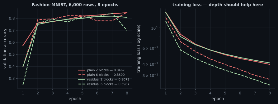
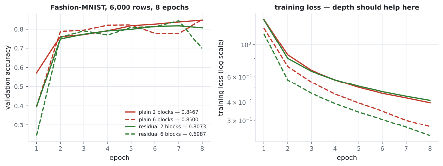
Does the shortcut help? Measured

The claim that made ResNet famous is that plain deep networks get worse with depth while residual ones keep improving. Tested at 4 and 12 convolutions:

figure Plain against residual at two depths matplotlib

The deeper models reach lower training loss in both families, so depth is helping the fit. On validation, plain 12 convolutions reached 0.8500 against residual's 0.8433, and the residual run's last epoch collapsed from a best of 0.8433 to 0.6987 — the instability is visible in the left panel. Depth helped the residual family more (+0.0260 against +0.0033) but from a lower starting point.

Model	Parameters	Best val accuracy	Final val	Final train loss	Seconds
plain, 4 convs	38,122	0.8467	0.8467	0.3953	117.0
plain, 12 convs	112,874	0.8500	0.8500	0.2701	262.4
residual, 4 convs	38,122	0.8173	0.8073	0.4105	117.6
residual, 12 convs	112,874	0.8433	0.6987	0.2339	235.4

The headline ResNet result did not reproduce, and it should not have. At twelve convolutions with batch normalisation there is no degradation problem to fix — the plain network trains perfectly well, reaching 0.8500. The shortcut has nothing to rescue.

What is visible is the direction of the effect:

• Depth helped the residual family eight times more (+0.0260 against +0.0033). Extrapolating that trend is exactly the argument the ResNet paper makes — it just needs tens of layers before the plain network starts losing.
• The residual model reached the lowest training loss (0.2339), so the shortcut is doing its job on optimisation; it is generalisation where it lost.
• The residual run was unstable at the end, dropping from 0.8433 to 0.6987 in one epoch. With shortcuts the effective learning rate on the residual branch is higher, and a fixed rate that suits the plain network can be too large here.

If you want to see the degradation ResNet fixes, you need 30+ layers, and on a CPU that is hours. The honest statement is: residual connections are insurance against depth, and at twelve layers you are not yet paying premiums.

The bug that made every number meaningless

The first version of this page reported validation accuracies of 0.11 to 0.20 while training loss sat at 0.30–0.46 — a model fitting its training data at ~85% and scoring near chance on validation.

The cause was not the architecture. Every model here uses batch normalisation, and at Keras’ default momentum=0.99 the moving statistics need roughly 460 batches to get within 1% of the truth — measured on the batch normalisation page. These runs are 6,000 rows at batch 128 for 8 epochs, which is 376 batches. The inference path was normalising with statistics that had never converged.

One argument, and the numbers became real

keras.layers.BatchNormalization(momentum=0.9)   # ~45 batches, not ~460

	Validation accuracy, plain 12 convs
momentum=0.99 (default), 376 batches	0.1540
momentum=0.9, 376 batches	0.8500

Same architecture, same data, same weights-in-training — a factor of five in the reported score, from one hyperparameter that has nothing to do with learning. Any short run with batch normalisation should lower the momentum, and any surprisingly bad validation score on a BN model should send you here first.

sketch Count a block's parameters p5.js Pause Restart

Build one block from each family and read the parameter count, computed with the same arithmetic Keras uses.

sketch The measured table, ranked p5.js Pause Restart

Click a column to rank every row by it. The bars are that column's values and the highest and lowest are computed from the numbers, not written in.

Pitfalls

• Putting the ReLU before a residual add. Activations then grow with depth and the deeper network gets worse — a bug that looks like a finding.
• Leaving BN at momentum=0.99 on a short run. It cost a factor of five in the reported validation accuracy here.
• Expecting ResNet’s headline at twelve layers. There is no degradation to fix until the plain network starts losing, which takes tens of layers.
• Reading a toy-scale ranking as an architectural verdict. Parameter count explained most of the ordering above.
• Running 5×5 branches at full resolution. Inception-ish was the slowest model here despite having 1×1 bottlenecks.
• Assuming separable convolutions always save 9×. The ceiling is the kernel area; measured savings ran 5.6× to 8.8×.
• Comparing architectures without holding the budget fixed. Same seed, same epochs, same data, or the comparison means nothing.

Recap

• The line runs LeNet → AlexNet → VGG → Inception → ResNet → Xception → SENet, each solving the previous step’s problem.
• Six miniatures on 6,000 rows: VGG-ish 0.8800 at 467,818 parameters, ResNet-ish 0.8173, LeNet-ish 0.7860, Inception-ish 0.6913, SENet-ish 0.6753, Xception-ish 0.5773 at 4,714 parameters.
• Depthwise-separable convolution saves 5.6× at 16 channels and 8.8× at 512, with the kernel area as the ceiling.
• Plain beat residual at both depths (0.8500 against 0.8433), but depth helped the residual family eight times more — the direction of the ResNet claim without the scale to demonstrate it.
• The residual model reached the lowest training loss and the least stable validation curve, collapsing 0.8433 → 0.6987 in one epoch.
• Batch normalisation at the default momentum made every validation number on this page meaningless until it was lowered to 0.9.

Next

Every model here was trained from random weights on a few thousand images. Starting from weights someone else already paid for changes the arithmetic completely: Transfer Learning Using Pre-trained Models.

pch.quizTag pch.quizDefaultTitle

1. A residual network's validation accuracy gets worse as you add blocks, while its training loss improves. You wrote the block as conv-BN-relu, then Add. What is wrong?

   A The shortcut needs a 1x1 convolution to match dimensions B The ReLU belongs after the merge, not before it — as written, the block adds non-negative values at every depth, so activations grow without bound as the network deepens C Residual connections require more than twelve layers to help D Batch normalisation should come after the ReLU
   pch.quizShowAnswer

   B — The ReLU belongs after the merge, not before it — as written, the block adds non-negative values at every depth, so activations grow without bound as the network deepens — The classic ordering is conv-BN-relu-conv-BN, then Add, then ReLU. This exact mistake produced a result that looked like evidence against ResNet.

2. Your BN-based model trains to 0.85 training accuracy but validates at 0.15 after 8 epochs on 6,000 rows at batch 128. What should you check first?

   A Whether the validation set is mislabelled B The BatchNormalization momentum — at the default 0.99 the moving statistics need about 459 batches to converge, and this run has only 376, so the inference path normalises with wrong statistics C Whether the learning rate is too high D Whether the model needs more regularisation
   pch.quizShowAnswer

   B — The BatchNormalization momentum — at the default 0.99 the moving statistics need about 459 batches to converge, and this run has only 376, so the inference path normalises with wrong statistics — Measured: 0.1540 at momentum=0.99 against 0.8500 at momentum=0.9, same architecture and data. Short runs should lower the momentum.

3. Xception-ish reached 0.5773 with 4,714 parameters while VGG-ish reached 0.8800 with 467,818. Which is the better architecture?

   A VGG-ish, because accuracy is what matters B Neither answer is available from this table alone — VGG-ish wins on accuracy and Xception-ish wins by two orders of magnitude on size, so the choice depends on whether you are constrained by accuracy or by bytes C Xception-ish, because efficiency always wins D They are equivalent once normalised by parameter count
   pch.quizShowAnswer

   B — Neither answer is available from this table alone — VGG-ish wins on accuracy and Xception-ish wins by two orders of magnitude on size, so the choice depends on whether you are constrained by accuracy or by bytes — Separable convolutions were designed for a deployment constraint. On a toy problem with no constraint, the bigger model simply wins.

4. Why do two stacked 3x3 convolutions appear everywhere after VGG?

   A Because 3x3 is the smallest kernel that can detect edges B Because they cover the same 5x5 receptive field as one 5x5 layer using 18 weights per channel pair instead of 25, and add an extra nonlinearity between them C Because GPUs only optimise 3x3 convolutions D Because larger kernels cannot be padded correctly
   pch.quizShowAnswer

   B — Because they cover the same 5x5 receptive field as one 5x5 layer using 18 weights per channel pair instead of 25, and add an extra nonlinearity between them — Fewer parameters and more nonlinearity for the same field. That single observation is most of VGG's contribution.

5. Depthwise-separable convolution saved 5.6x at 16 channels and 8.8x at 512. Why does the saving grow, and what is its limit?

   A It grows without limit as channels increase B The standard cost is quadratic in channels while the depthwise part is linear, so the ratio approaches the kernel area — 9 for a 3x3 kernel — without ever reaching it C It is limited by the number of filters, not the kernel D The saving is constant and the measurements are noise
   pch.quizShowAnswer

   B — The standard cost is quadratic in channels while the depthwise part is linear, so the ratio approaches the kernel area — 9 for a 3x3 kernel — without ever reaching it — Standard is k^2*Cin*Cout; separable is k^2*Cin + Cin*Cout. As Cout grows the first term stops mattering and the ratio tends to k^2.

🧪 Try It Yourself

pch.exerciseTag pch.exerciseTitle

pch.exerciseTag pch.exerciseTitle

pch.exerciseTag pch.exerciseTitle

pch.exerciseTag pch.exerciseTitle

pch.exerciseTag pch.exerciseTitle