Loading & Preprocessing Data with tf.data

Input-pipeline advice usually arrives as a list of methods to chain in a particular order: map, cache, shuffle, batch, prefetch. Every item on that list is a throughput claim, and throughput is measurable, so this page times each one instead of repeating the list.

The measurements use a deliberately slow map function — four average-pooling passes plus noise per image. That choice matters: on a pipeline whose per-sample work is trivial, every option looks identical and the page would teach nothing.

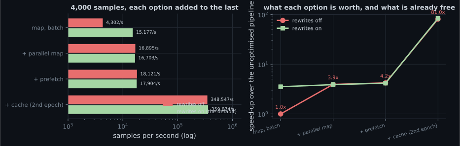
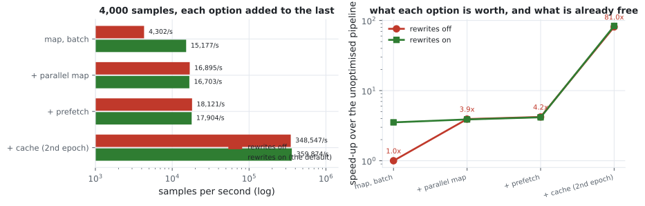
Pipeline	Rewrites off	Speed-up	Rewrites on (default)	Speed-up
map, batch	4,302/s	1.00×	15,177/s	3.53×
+ num_parallel_calls	16,895/s	3.93×	16,703/s	3.88×
+ prefetch	18,121/s	4.21×	17,904/s	4.16×
+ cache (2nd epoch)	348,547/s	81.01×	359,874/s	83.64×

The second column pair is the surprise. tf.data already rewrote the plain map into a parallel one before being asked, which is why adding num_parallel_calls measures 3.88× against a default that was already at 3.53×. The advice is not wrong — it is mostly already applied.

What you’ll learn

• What each pipeline option is worth on this machine, and which ones tf.data applies for you.
• Why cache is in a completely different league (81×) from everything else.
• What prefetch actually fixes, measured as time spent waiting rather than as throughput.
• Why the batch-size sweep came out flat, against the usual expectation.

The graph rewrites you did not ask for

Turning the automatic optimisations off, to see what they were doing

options = tf.data.Options()
options.experimental_optimization.map_parallelization = False
options.experimental_optimization.map_and_batch_fusion = False
options.autotune.enabled = False
pipeline = pipeline.with_options(options)

tf.data compiles your pipeline into a graph and rewrites it. A stateless map becomes a parallel map; a map followed by a batch may be fused into one operation. Those rewrites are on by default, and they account for the jump from 4,302/s to 15,177/s in the table above without a single line of user code.

This has a practical consequence: benchmarking a pipeline option on modern tf.data usually measures nothing, because the runtime already did it. To find out what an option is worth you have to switch the rewrites off, which is what the first column pair does.

figure 4,000 MNIST images through a deliberately expensive map matplotlib

The two lines converge as soon as num_parallel_calls is set explicitly, because at that point the user has asked for what the rewrite was already doing. The gap on the first row — 3.53x — is the value tf.data adds silently. The last row dwarfs everything: caching a computed epoch is 81x, because the second pass does no work at all.

Cache is not in the same category

Everything except cache is about overlapping work. Caching removes the work entirely: on the second epoch the expensive map has already run, and the pipeline is only replaying arrays from memory. 348,547 samples per second is not a faster pipeline; it is the absence of a pipeline.

Two conditions make it safe, and both are easy to get wrong:

• The data must fit. cache() with no argument holds everything in RAM. cache("path") spills to disk, which is slower but survives a dataset larger than memory.
• The cached step must be deterministic. Caching after random augmentation freezes one augmentation per sample forever — the model then sees the same “random” crops every epoch, which quietly removes the regularisation you were paying for.

Where cache goes relative to augmentation

# Right: deterministic work cached, randomness applied fresh each epoch.
pipeline = (raw.map(decode_and_resize, num_parallel_calls=AUTOTUNE)
               .cache()
               .map(random_augment, num_parallel_calls=AUTOTUNE)
               .batch(64).prefetch(AUTOTUNE))

That the numbers here were timed on the second pass is also deliberate. The first pass has to do the work before there is anything to cache, so timing it would report the cost and hide the benefit.

Prefetch, measured properly

Throughput is the wrong test for prefetch. In the table above it contributes 4.21× against the parallel map’s 3.93× — barely anything — because when nothing is consuming the data there is nothing to overlap with.

The right test simulates a training step and measures how long the consumer spends waiting:

figure A 3 ms busy-wait standing in for the training step matplotlib

The step is a busy-wait rather than a sleep, so it cannot overlap by accident the way a sleeping thread would. Prefetch cut waiting from 24.8% of the epoch to 18.3% — real, and much smaller than the usual telling suggests, because the parallel map was already running ahead of the consumer. The remaining wait is the first batch, which nothing can overlap.

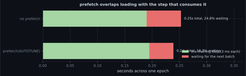
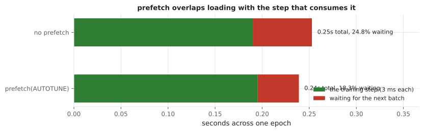
prefetch does not make loading faster. It makes loading happen while the previous batch is being trained on. The measurement to watch is the share of wall-clock the consumer spends blocked, and here that share was already low before prefetch was added.

diagram Diagram mermaid

  flowchart LR
  R["raw samples"] --> M["map: the expensive part"]
  M --> C["cache: skip it entirely
on later epochs (81x)"]
  C --> S["shuffle"]
  S --> B["batch"]
  B --> P["prefetch: overlap with
the training step"]
  P --> T["training step"]
  M -.->|"parallel map, 3.93x"| W["8 workers on 8 cores"]
  T -.->|"24.8% waiting -> 18.3%"| Q["is the consumer starved?"]

Parallelism, and where AUTOTUNE landed

figure This machine has 8 logical cores matplotlib

The parallelism curve is the clean result: 4,511 samples per second on one worker rising to 16,701 on eight, a 3.7x gain on 8 cores. AUTOTUNE landed at 14,641 — below the best explicit setting in this run, which is worth knowing: it adapts at run time and a short single-epoch measurement does not give it long to converge. The batch-size panel is flat, which is the honest result rather than a broken measurement.

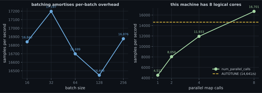
Workers	Samples/s
1	4,511
2	8,050
4	11,933
8	16,701
AUTOTUNE	14,641

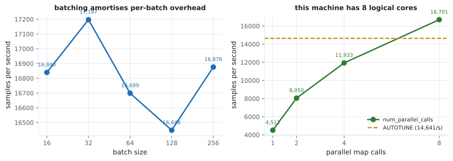
Scaling from 1 to 8 workers gave 3.7× on 8 logical cores — close to linear until the last doubling, where the cores are also running the main thread and TensorFlow’s own thread pools.

AUTOTUNE came in below the best fixed setting here. That is not a reason to abandon it: it tunes at run time across a whole training job, and these measurements are single passes over 4,000 samples. But it is a reason to distrust “AUTOTUNE is always optimal” and to measure if the input pipeline is your bottleneck.

The batch-size result

Batch size	16	32	64	128	256
Samples/s	16,840	17,197	16,699	16,448	16,876

Flat, within noise, across a 16× range. Batching amortises per-batch overhead, and on this pipeline that overhead is negligible next to the map — so there is nothing to amortise.

This is worth stating because “use a bigger batch for throughput” is common advice. It is about the training step, where a bigger batch means better hardware utilisation, not about the input pipeline. Measuring the two separately is what keeps the claims straight.

sketch Serial against overlapped p5.js Pause Restart

Drag the loading time. The top track loads then trains, one after the other; the bottom track loads the next batch while training on the current one.

sketch The measured table, ranked p5.js Pause Restart

Click a column to rank every row by it. The bars are that column's values and the highest and lowest are computed from the numbers, not written in.

Pitfalls

• Benchmarking an option without disabling the rewrites. Adding num_parallel_calls measured 3.88× against a default of 3.53× — almost all of it was already applied.
• Caching after random augmentation. The randomness is frozen on the first epoch, silently removing the regularisation.
• Timing cache on the first pass. That pass pays the cost and gets none of the benefit.
• Judging prefetch by throughput. It contributes almost nothing there; its effect is on consumer waiting time, 24.8% → 18.3%.
• Assuming AUTOTUNE beats a fixed setting. It scored 14,641 against 16,701 for eight explicit workers in this run.
• Expecting bigger batches to raise pipeline throughput. Flat from 16 to 256 here.
• Benchmarking with a trivial map. Every option looks free, which is why so much pipeline advice is passed on untested.

Recap

• tf.data rewrites your pipeline before running it; a stateless map is parallelised for you, worth 3.53× here.
• Explicit num_parallel_calls reached 3.93×, so the manual version adds little over the default.
• cache is categorically different at 81×, because the second epoch does no work — but only if the data fits and the cached stage is deterministic.
• prefetch overlaps loading with the training step; measured as waiting time it went 24.8% → 18.3%.
• Parallel map scaling was 4,511 → 16,701 samples per second from 1 to 8 workers.
• Batch size did not affect pipeline throughput at all on this workload.

Next

With data arriving fast enough, the next bottleneck is the training step itself — and the fit() loop can be replaced with one you write: Custom Models and Training Loops.

pch.quizTag pch.quizDefaultTitle

1. The plain map ran at 4,302 samples/s with graph rewrites off and 15,177 with them on. What does that mean for pipeline benchmarking?

   A The rewrites make measurements unreliable B tf.data already parallelises a stateless map for you, so measuring 'the benefit of num_parallel_calls' on default settings mostly measures nothing — the rewrite had already applied it C The rewrites should always be disabled D The map function was stateful
   pch.quizShowAnswer

   B — tf.data already parallelises a stateless map for you, so measuring 'the benefit of num_parallel_calls' on default settings mostly measures nothing — the rewrite had already applied it — Adding num_parallel_calls explicitly reached 3.93x against a default that was already at 3.53x.

2. Caching gave 81x while every other option gave around 4x. Why is it in a different category?

   A It uses a faster memory allocator B The other options overlap or parallelise the work; cache removes it — on the second epoch the expensive map has already run and the pipeline just replays arrays C It skips the batching step D It compresses the data
   pch.quizShowAnswer

   B — The other options overlap or parallelise the work; cache removes it — on the second epoch the expensive map has already run and the pipeline just replays arrays — That is also why it must be timed on the second pass: the first one pays the full cost and has nothing cached yet.

3. Why is caching AFTER a random augmentation step a bug?

   A It uses more memory B The augmentation is executed once and its result stored, so every later epoch sees the identical 'random' transformation — the regularisation silently disappears C Augmentation cannot be serialised D It makes the pipeline non-deterministic
   pch.quizShowAnswer

   B — The augmentation is executed once and its result stored, so every later epoch sees the identical 'random' transformation — the regularisation silently disappears — Cache belongs after the deterministic work — decoding, resizing — and before anything that should differ each epoch.

4. Prefetch added almost nothing to raw throughput but cut consumer waiting from 24.8% to 18.3%. What does prefetch actually do?

   A It loads data faster B It overlaps loading with the training step that consumes the previous batch, so throughput of the pipeline alone is the wrong measurement for it C It increases the batch size automatically D It caches the first few batches
   pch.quizShowAnswer

   B — It overlaps loading with the training step that consumes the previous batch, so throughput of the pipeline alone is the wrong measurement for it — With nothing consuming the data there is nothing to overlap with, which is why the throughput table barely moves.

5. Batch size made no difference to pipeline throughput (16,448 to 17,197 across a 16x range). Is the common 'use bigger batches' advice wrong?

   A Yes, batch size never matters B No — that advice is about the training step, where a larger batch improves hardware utilisation; here the map dominates and there is no per-batch overhead left to amortise C Yes, because the measurement was too noisy D No, but only because this ran on a CPU
   pch.quizShowAnswer

   B — No — that advice is about the training step, where a larger batch improves hardware utilisation; here the map dominates and there is no per-batch overhead left to amortise — Measuring the input pipeline and the training step separately is what keeps the two claims from being confused.

🧪 Try It Yourself

pch.exerciseTag pch.exerciseTitle

pch.exerciseTag pch.exerciseTitle

pch.exerciseTag pch.exerciseTitle

pch.exerciseTag pch.exerciseTitle

pch.exerciseTag pch.exerciseTitle

pch.exerciseTag pch.exerciseTitle