The Transformer Architecture

A transformer block is four things stacked: layer normalisation, multi-head attention, a residual connection, and a small feed-forward network — with another norm and residual around it. The attention page measured the attention. This page measures everything around it, by removing one piece at a time.

The result is uncomfortable and worth confronting directly: at one block, every single ablation improved the score.

Setting	Parameters	Best validation accuracy	vs full
full block	328,577	0.8462	—
no positional embeddings	328,577	0.8405	−0.0058
no feed-forward	324,321	0.8515	+0.0052
no residuals	328,577	0.8562	+0.0100
no layer normalisation	328,449	0.8665	+0.0203

The full block was the worst configuration tested. Rather than explain that away, the page repeats the experiment at depth — where the answer changes for one component and does not for another.

What you’ll learn

Where a block’s parameters actually live: 95.54% of them are the token embedding.
The measured comparison against recurrence, including a transformer that reaches its best accuracy in epoch 1.
What each component contributes at one block — all of them negative except positions.
What changes at four blocks: removing layer norm costs 0.0612, while removing residuals still does not hurt.
Why the pooled-output design makes the positional ablation a measurement of the task, not the architecture.

The block, and where its parameters go

A pre-norm transformer block

def block(x, width, heads):
    normed = keras.layers.LayerNormalization(epsilon=1e-6)(x)
    attention = keras.layers.MultiHeadAttention(num_heads=heads,
                                                key_dim=width // heads)(normed, normed)
    x = keras.layers.Add()([x, attention])                       # residual
    normed = keras.layers.LayerNormalization(epsilon=1e-6)(x)
    hidden = keras.layers.Dense(width * 2, activation="relu")(normed)
    return keras.layers.Add()([x, keras.layers.Dense(width)(hidden)])   # residual

Component	Parameters	Share
token embedding	320,000	95.54%
position embedding	6,400	1.91%
attention (Q, K, V, out)	4,224	1.26%
feed-forward	4,192	1.25%
layer norms (×2)	128	0.04%
total	334,944

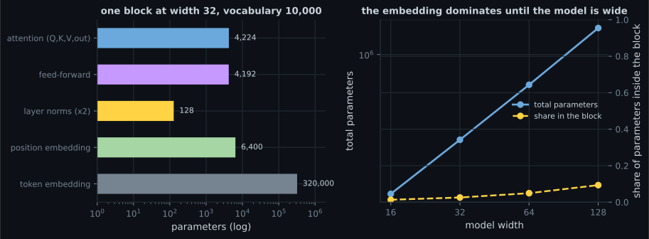
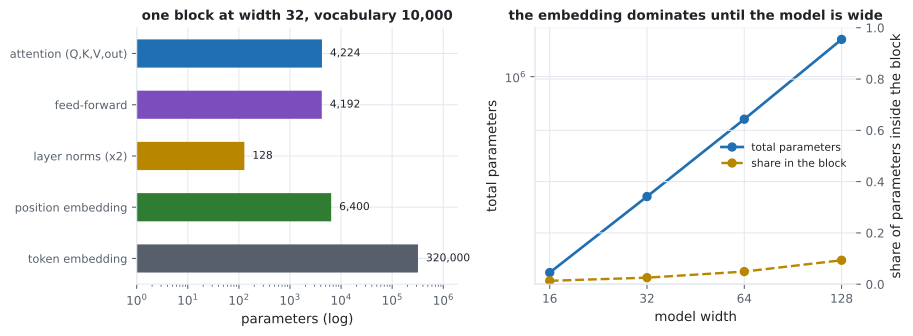
figure One block at width 32, vocabulary 10,000 matplotlib

At this scale the model is an embedding table with a transformer attached. Attention — the part the architecture is named for — is 1.26% of the parameters, and both layer norms together are 128 numbers. The right panel shows why large models look different: block parameters grow with width squared while the embedding grows linearly, so the ratio inverts as models get wide.

This matters for reading the ablations below. Removing the feed-forward network deletes 1.25% of the parameters; removing both layer norms deletes 0.04%. These are not capacity experiments — they are experiments about optimisation.

Against recurrence

Family	Parameters	Best validation accuracy	Seconds	Epoch 1
bag of words	320,033	0.8465	39.1	0.7303
GRU	326,369	0.8210	214.9	0.8018
LSTM	328,353	0.8415	264.9	0.8130
transformer	328,577	0.8462	383.5	0.8462

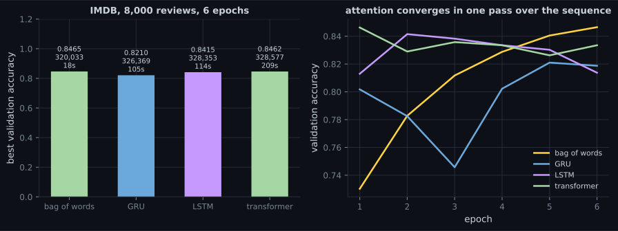
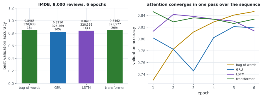
Two panels. Left: bars of best validation accuracy for four families, all between 0.8210 and 0.8465, annotated with parameters and training seconds. Right: per-epoch validation accuracy where the transformer starts at 0.8462 in epoch one and stays flat, while the bag of words climbs from 0.7303 and the recurrent models rise more slowly. — The transformer's entire learning happens in epoch 1 — 0.8462, which is also its best score across all six epochs. Attention over 200 positions in parallel means every token pair is one gradient step apart, so there is no long credit-assignment chain to unroll. That is the real advantage on display here; it is not accuracy, since the bag of words matched it at 0.8465 in a tenth of the time.

The transformer’s −0.0002 against a bag of words is the same lesson as the sentiment bake-off: on this task, at this scale, architecture is not the binding constraint. What is visible is convergence speed — one epoch against six.

The ablations, at one block

figure Remove one piece at a time — 6 epochs, width 32 matplotlib

Only the positional embeddings earn their place at this depth, and only barely (-0.0058 when removed). Everything else is dead weight or worse: the full block is the lowest bar except for the positionless variant. The honest reading is that residuals, the feed-forward network and normalisation are not there to raise the accuracy of a one-block model — and the next figure tests what they *are* there for.

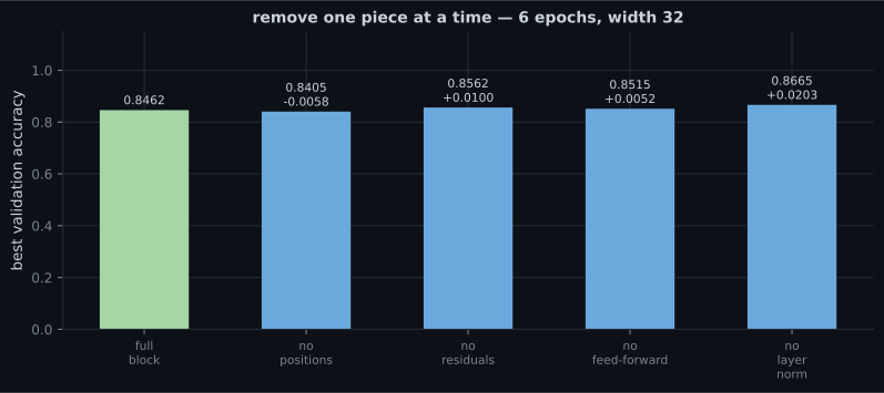
The positional ablation measures the task

Removing positions cost only 0.0058, and the reason is structural: this classifier ends with GlobalAveragePooling1D. Averaging is permutation-invariant, so with no positional information the whole model becomes a bag of words with an attention-weighted average inside it — and the bag of words scores 0.8465. The ablation is therefore a measurement of how much sentiment needs word order, which the intro-to-RNNs page put at +0.0744 for a recurrent model and +0.0000 for averaging.

For a generative transformer this ablation is not available: without positions a language model cannot tell the cat sat from sat cat the, and its loss would reflect that immediately.

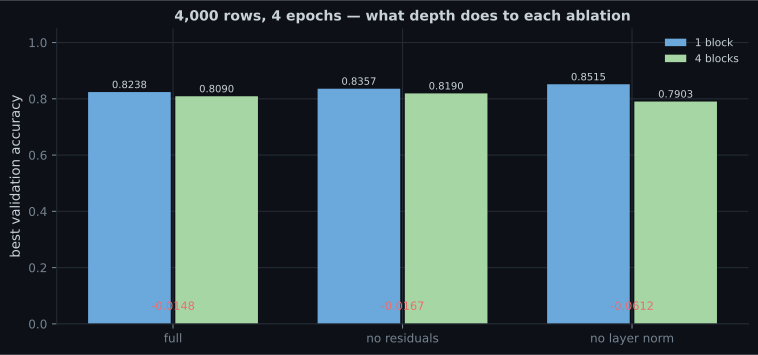
The same ablations at depth

If residuals and normalisation exist to make deep stacks trainable, then the deep column should punish removing them. Same code, 1 block against 4:

Setting	1 block	4 blocks	Deep − shallow
full	0.8238	0.8090	−0.0148
no residuals	0.8357	0.8190	−0.0167
no layer normalisation	0.8515	0.7903	−0.0612

Grouped bars comparing one block against four blocks for three settings. Full scores 0.8238 and 0.8090; no residuals 0.8357 and 0.8190; no layer norm 0.8515 at one block but collapses to 0.7903 at four, annotated with a change of -0.0612. — Layer normalisation behaves exactly as advertised: free to remove at one block (the best score in the shallow column) and the worst configuration at four, losing 0.0612 where the full block loses 0.0148. Residual connections do not reproduce that pattern here — they are still marginally better removed at four blocks. Four is not deep; the residual argument is about dozens of layers, and this phase cannot afford to run that.

Two conclusions, stated at the strength the data supports:

Layer normalisation’s value is depth. At one block it is 128 wasted parameters; at four blocks it is the difference between 0.8090 and 0.7903. That is a direct confirmation, and it is why every transformer has it.
Residual connections are not vindicated at four blocks. They remain slightly negative. The published argument for residuals concerns dozens of layers, where the gradient path length is the binding problem — the same claim the ResNet page also failed to reproduce at 12 convolutions. Two independent failures to reproduce at small depth, in the same direction, is consistent with the claim being about scale rather than being wrong.

diagram Diagram mermaid

  flowchart TB
  A["tokens"] --> B["embedding + positions"]
  B --> C["LayerNorm"]
  C --> D["MultiHeadAttention"]
  D --> E["+ residual"]
  B --> E
  E --> F["LayerNorm"]
  F --> G["Dense -> Dense"]
  G --> H["+ residual"]
  E --> H
  H --> I["GlobalAveragePooling1D"]
  I --> J["Dense 1, sigmoid"]
  K["at 1 block: every removal helps"] -.-> H
  L["at 4 blocks: removing LayerNorm costs 0.0612"] -.-> H

sketch Where the parameters are p5.js

Drag the model width. The block's parameters grow with the square of the width while the embedding grows linearly, so the balance flips.

sketch The measured table, ranked p5.js

Click a column to rank every row by it. The bars are that column's values and the highest and lowest are computed from the numbers, not written in.

Pitfalls

Assuming every component raises accuracy. At one block, four of five ablations scored higher than the full block.
Concluding the components are useless. Layer normalisation went from best-when- removed at 1 block to worst at 4, costing 0.0612.
Reading an ablation as a capacity test. Both layer norms are 128 parameters — 0.04% of the model. What changes is optimisation, not capacity.
Ablating positions on a pooled classifier and calling it an architecture result. Average pooling is permutation-invariant, so that ablation measures the task’s need for word order.
Post-norm without warmup. This page uses pre-norm throughout; Add then normalise needs a learning-rate schedule to train at all.
Comparing architectures on accuracy alone. The transformer matched a bag of words (−0.0002) at 10× the cost, but reached its best score in epoch 1 against six.
Calling this a transformer result. One block, width 32, trained from scratch on 8,000 reviews is not what the papers measure.

Recap

A block is pre-norm → attention → residual → pre-norm → feed-forward → residual.
At width 32 with a 10,000-word vocabulary, 95.54% of parameters are the token embedding; attention is 1.26% and both norms are 0.04%.
Against recurrence: bag of words 0.8465, GRU 0.8210, LSTM 0.8415, transformer 0.8462 — but the transformer reached its best in epoch 1.
At one block every ablation but positions improved the score, with no-layer-norm best at 0.8665.
At four blocks removing layer norm cost 0.0612 against the full block’s 0.0148 — the component’s value is depth.
Residuals stayed marginally positive-to-remove even at four blocks; that argument is about dozens of layers.

An encoder reads a sequence. Producing a different sequence needs a decoder, teacher forcing, and attention between the two: Sequence-to-Sequence Learning (Machine Translation).

pch.quizTag pch.quizDefaultTitle

At one block, removing layer normalisation improved accuracy from 0.8462 to 0.8665. At four blocks it dropped it to 0.7903 against the full block's 0.8090. What does that show?

pch.quizShowAnswer

B — Its value is depth — it is 128 spare parameters in a shallow model and the difference between training and not training in a deeper one — This is why the ablation was repeated at depth instead of explaining the shallow result away: the prediction was specific and it held.
At width 32 with a 10,000-word vocabulary, what fraction of a one-block transformer's parameters is the attention mechanism?

pch.quizShowAnswer

B — 1.26% — the token embedding is 95.54%, so at this scale the model is an embedding table with a transformer attached — Block parameters grow with width squared while the embedding grows linearly, so the ratio inverts in large models.
Removing the positional embeddings cost only 0.0058. Why is that not an argument against positional encoding?

pch.quizShowAnswer

B — Because the classifier ends in average pooling, which is permutation-invariant — so the ablation measures how much sentiment needs word order, not whether positions matter architecturally — A generative transformer cannot run this ablation at all: without positions it could not distinguish 'the cat sat' from 'sat cat the'.
The transformer scored 0.8462 and reached that in epoch 1, while the LSTM reached 0.8415 over six epochs. What is the real advantage on display?

pch.quizShowAnswer

B — Convergence speed — every token pair is one gradient step apart under attention, so there is no long credit-assignment chain to unroll — On accuracy the transformer tied a bag of words at -0.0002 while costing ten times as much wall-clock.
Residual connections were still slightly better removed even at four blocks. What is the appropriate conclusion?

pch.quizShowAnswer

B — Four blocks is not deep — the published argument concerns dozens of layers, and this phase also failed to reproduce the ResNet claim at 12 convolutions, both in the same direction — Two independent failures to reproduce at small depth, both pointing the same way, is consistent with the claim being about scale rather than being false.

🧪 Try It Yourself

pch.coffeeTagline

pch.coffeeCta

pch.feedbackHeading

pch.feedbackSubheading