
Introduction to Neural Networks (The Perceptron)
Every deep network is built from one unit: multiply each input by a weight, add them up, add a bias, and pass the total through an activation. This page takes that unit as far as it goes — which is exactly one straight line — proves where it stops, and fixes it with nine parameters.
What you’ll learn
Section titled “What you’ll learn”- The perceptron’s forward pass and its 1958 learning rule, both written out and run.
- Why it converges on AND in 9 epochs and never converges on XOR, measured.
- A four-line proof by contradiction that no straight line can compute XOR.
- Exactly 14 of the 16 two-input boolean functions a single perceptron can learn — enumerated, not asserted.
- The two-layer XOR construction, with weights you can check by hand.
- Why the step function makes gradient descent impossible, and what replaced it.
One neuron, written out
Section titled “One neuron, written out”For inputs , weights and a bias :
The geometry is the whole story. is a hyperplane — a line in 2D, a plane in 3D. is the direction perpendicular to it, and decides how far from the origin it sits: the distance is . Everything on one side outputs 1; everything on the other outputs 0. A perceptron is a line, and a decision about which side you are on.
  flowchart LR
  X1["x1"] -->|"w1"| SUM["z = w1x1 + w2x2 + b"]
  X2["x2"] -->|"w2"| SUM
  B["1"] -->|"b"| SUM
  SUM --> ACT{{"step: is z greater than 0?"}}
  ACT -->|"yes"| Y1["output 1"]
  ACT -->|"no"| Y0["output 0"]
The learning rule
Section titled “The learning rule”Rosenblatt’s 1958 rule visits one row at a time and only acts when it is wrong:
There are only three cases. Prediction correct, : nothing moves. Predicted 0 when the answer was 1, : add , pushing up for this input. Predicted 1 when the answer was 0: subtract, pushing down. That is the entire algorithm — no derivatives, no loss function.
import numpy as np

def perceptron(X, y, lr=0.1, max_epochs=100, seed=0):
    """Rosenblatt's rule. Returns whether it separated the data, and in how many passes."""
    rng = np.random.default_rng(seed)
    w, b = rng.normal(0, 0.01, X.shape[1]), 0.0
    for epoch in range(1, max_epochs + 1):
        errors = 0
        for xi, target in zip(X, y):
            prediction = 1 if xi @ w + b > 0 else 0
            step = lr * (target - prediction)          # +lr, -lr, or exactly 0
            if step != 0:
                w, b, errors = w + step * xi, b + step, errors + 1
        if errors == 0:                                 # a full clean pass
            return {"converged": True, "epochs": epoch, "w": w, "b": b}
    return {"converged": False, "epochs": max_epochs, "w": w, "b": b}
The Perceptron Convergence Theorem guarantees this halts if the data is linearly separable. Note what it does not promise: nothing about the quality of the line, and nothing at all when the data is not separable.
Run it on the four gates
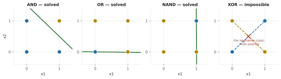
Section titled “Run it on the four gates”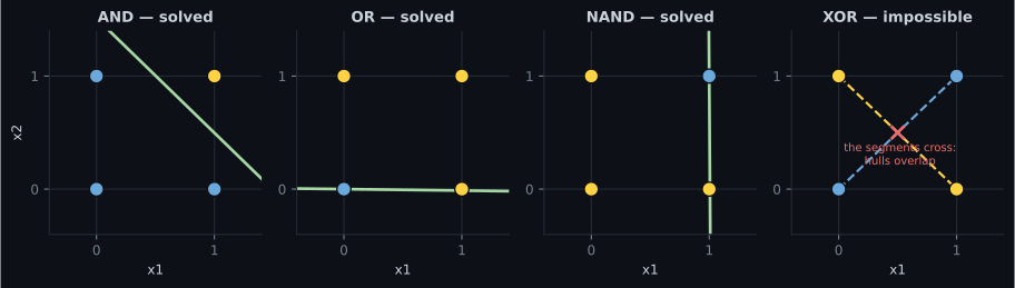
| Gate | Outcome | Final weights | Bias |
|---|---|---|---|
| AND | converged in 9 epochs | [+0.201, +0.199] | −0.30 |
| OR | converged in 3 epochs | [+0.001, +0.099] | +0.00 |
| NAND | converged in 4 epochs | [−0.199, −0.001] | +0.20 |
| XOR | never converged (stopped at 100) | [−0.199, −0.001] | +0.10 |
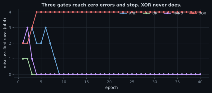
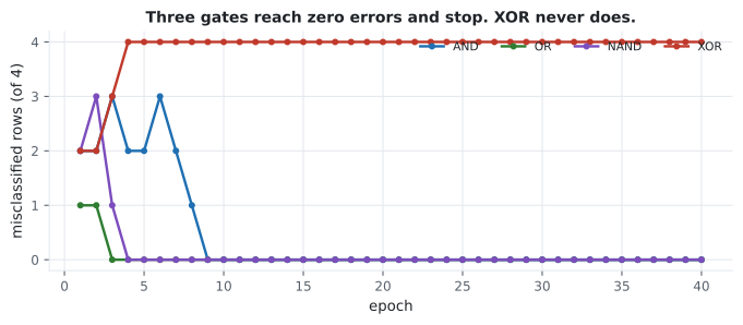
The convergence plot shows one run failing. A stronger statement is available cheaply: search every single neuron and check that none of them works.
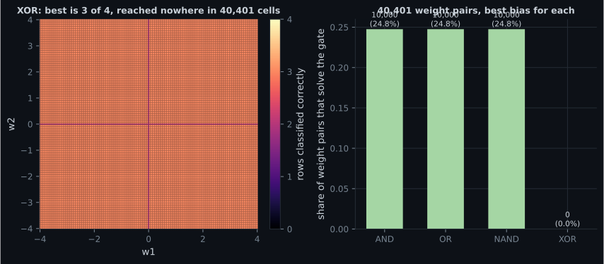
| Gate | Best of 4 rows | Weight pairs that solve it | Share |
|---|---|---|---|
| AND | 4 | 10,000 | 24.75% |
| OR | 4 | 10,000 | 24.75% |
| NAND | 4 | 10,000 | 24.75% |
| XOR | 3 | 0 | 0.00% |
Look at OR’s weights: , . That line passes within 0.001 of two of its four data points. It is a valid separator, so the algorithm stopped — the perceptron takes the first line that works, not the best one. That is precisely the gap support vector machines close by maximising the margin instead.
Why XOR is impossible
Section titled “Why XOR is impossible”Suppose weights and bias exist with exactly when . Write down what each row demands:
| Row | Target | Constraint |
|---|---|---|
| 0 | ||
| 1 | ||
| 1 | ||
| 0 |
Add rows 2 and 3: , so . Row 4 says . Together:
which contradicts row 1. No such exists — for a perceptron or for any linear classifier, at any learning rate, with any amount of data.
So how many boolean functions can one neuron learn?
Section titled “So how many boolean functions can one neuron learn?”Two inputs give possible truth tables. Running the rule on every one of them:
14 of 16 are learnable. The two that are not are exactly (XOR) and (XNOR).
That reframes the 1969 objection usefully. A single neuron is not weak in general — it handles 87.5% of two-input logic. It fails on precisely the functions whose positive examples sit on one diagonal, and that is a statement about geometry, not capacity.
The two-layer fix, by hand
Section titled “The two-layer fix, by hand”XOR is “OR, but not AND”, which is expressible as — and each of those three is linearly separable. Wire them in two layers with a hidden layer of two units:
Hidden unit 1 computes , which is OR. Hidden unit 2 computes , which is NAND. The output computes , which is AND. Every row:
| (OR) | (NAND) | output | XOR | ||
|---|---|---|---|---|---|
| 0 | 0 | 0 | 1 | 0 | 0 |
| 0 | 1 | 1 | 1 | 1 | 1 |
| 1 | 0 | 1 | 1 | 1 | 1 |
| 1 | 1 | 1 | 0 | 0 | 0 |
Exact match, using 9 parameters and no training at all. The hidden layer’s job is to re-represent the input so that the output layer’s straight line becomes sufficient — which is what every hidden layer in every deep network is doing.
The step function cannot be trained by gradient descent
Section titled “The step function cannot be trained by gradient descent”Gradient descent needs , and the chain rule routes that through :
| numeric derivative | ||
|---|---|---|
| −2.0 | 0 | 0.0 |
| −0.1 | 0 | 0.0 |
| +0.1 | 1 | 0.0 |
| +2.0 | 1 | 0.0 |
Every update becomes . The weights never move. This is why Rosenblatt needed a bespoke rule, and why the smooth sigmoid — whose derivative reaches 0.25, as measured on the activations page — was the change that made backpropagation possible.
Swapping the step for a sigmoid turns the same unit into something trainable:
from tensorflow import keras

# One neuron, two inputs. The only change from a TLU is the activation.
model = keras.Sequential([
    keras.layers.Input((2,)),
    keras.layers.Dense(1, activation="sigmoid"),
])
model.compile(loss="binary_crossentropy", optimizer="sgd", metrics=["accuracy"])
On real data
Section titled “On real data”Two MNIST digit pairs, 2,000 training rows each, the perceptron rule against a single sigmoid unit trained for 20 epochs:
| Task | Perceptron | Test accuracy | Sigmoid unit |
|---|---|---|---|
| 0 vs 1 | separated the training set | 0.9976 | 1.0000 |
| 3 vs 5 | never separated it | 0.9663 | 0.9508 |
| 4 vs 9 | never separated it | 0.9513 | 0.9635 |
Two things worth noticing. Handwritten 0s and 1s are close to linearly separable in raw pixel space, which is why the rule terminates and both models are near-perfect. And on 3 vs 5 the perceptron beat the sigmoid unit (0.9663 against 0.9508) despite never converging — non-convergence means “no line separates the training set”, not “the line is useless”. Failing to converge is information about your data.
See it move
Section titled “See it move”The second sketch is the learning rule itself. Each click applies one epoch of updates; the line moves only on rows it gets wrong. Switch to XOR and watch it never settle.
Pitfalls
Section titled “Pitfalls”Expecting non-convergence to be a bug. If the data is not linearly separable the rule cannot terminate, by construction. The fix is a different model, not more epochs.
Reading the perceptron’s line as a good line. It stops at the first separator it finds. The OR run above ended with a boundary 0.001 away from two of its four points.
Using the step function with gradient descent. Its derivative is 0 everywhere, so the update is exactly zero. Any modern “perceptron” you train with an optimiser has a sigmoid or ReLU in it, not a step.
Assuming a bias-free neuron is only slightly weaker. Without , the boundary must pass through the origin. AND is unlearnable in that setting: every row of the truth table would need to be false at , which is already forced.
Believing the 1969 objection killed the idea because a neuron is weak. One neuron learns 14 of the 16 two-input functions. Two layers and 9 parameters cover the other two. What was missing for another 17 years was a way to train the second layer.
- A perceptron is : a hyperplane, plus a decision about which side you are on.
- The rule only fires on mistakes, and converged in 9, 3 and 4 epochs on AND, OR and NAND.
- XOR is impossible for any linear classifier — the four constraints force and at once.
- 14 of 16 two-input boolean functions are learnable by one neuron; the exceptions are XOR and XNOR.
- Two layers, 9 parameters, no training: OR and NAND in the hidden layer, AND on top, exactly reproducing XOR.
- everywhere, which is why sigmoid replaced it and why backpropagation had to wait.
- On 3 vs 5 MNIST digits the non-converged perceptron scored 0.9663 against a sigmoid unit’s 0.9508 — non-convergence describes the data, not the quality of the answer.
-
The perceptron rule runs for 100 epochs on XOR and never converges. What should you conclude?
The Perceptron Convergence Theorem only guarantees termination for linearly separable data. The contradiction proof on this page rules out every possible line, so tuning cannot help. Two layers and 9 parameters can.
pch.quizShowAnswer
B — XOR is not linearly separable, so no setting of any hyperparameter will make it converge — the four truth-table constraints force b > 0 and b <= 0 simultaneously — The Perceptron Convergence Theorem only guarantees termination for linearly separable data. The contradiction proof on this page rules out every possible line, so tuning cannot help. Two layers and 9 parameters can.
-
How many of the 16 two-input boolean functions can a single perceptron learn?
A single neuron is not weak in general; it fails on precisely the two functions whose positive examples sit on opposite diagonals, which is a geometric property rather than a capacity limit.
pch.quizShowAnswer
B — 14 — every function except XOR [0,1,1,0] and XNOR [1,0,0,1], which was verified by running the rule on all 16 truth tables — A single neuron is not weak in general; it fails on precisely the two functions whose positive examples sit on opposite diagonals, which is a geometric property rather than a capacity limit.
-
Why can gradient descent not train a step-function neuron?
The chain rule multiplies by step'(z) = 0, so every update is exactly zero. This is why Rosenblatt needed a bespoke rule and why the smooth sigmoid — derivative up to 0.25 — was the change that unlocked backpropagation.
pch.quizShowAnswer
B — Its derivative is 0 for every z except 0 (where it is undefined), so w -= lr * grad leaves every weight exactly where it was — The chain rule multiplies by step'(z) = 0, so every update is exactly zero. This is why Rosenblatt needed a bespoke rule and why the smooth sigmoid — derivative up to 0.25 — was the change that unlocked backpropagation.
-
The measured OR run ended with w = [+0.001, +0.099] and b = 0.00, a boundary passing within 0.001 of two data points. What does that tell you about the algorithm?
Zero errors is the stopping condition, so any separating line ends training. A boundary that grazes the data generalises worse than a centred one, which is the gap the max-margin objective closes.
pch.quizShowAnswer
B — It stops at the first line that separates the data, not the best one — maximising the margin instead is exactly what an SVM adds — Zero errors is the stopping condition, so any separating line ends training. A boundary that grazes the data generalises worse than a centred one, which is the gap the max-margin objective closes.
-
In the two-layer XOR construction, what is the hidden layer doing?
Both hidden units compute linearly separable functions of the raw input. In their output space the two XOR-positive rows both become (1,1), so the output neuron's straight line suffices. Every hidden layer in every deep network is doing this.
pch.quizShowAnswer
B — Re-representing the input as (OR, NAND), a space in which a single straight line — AND — is enough — Both hidden units compute linearly separable functions of the raw input. In their output space the two XOR-positive rows both become (1,1), so the output neuron's straight line suffices. Every hidden layer in every deep network is doing this.
You have taken one neuron as far as it goes, and seen the two-layer fix built by hand. Continue to Multi-Layer Perceptron (MLP) to stack these units properly and see how the hidden layer’s re-representation is learned rather than hand-designed.
🧪 Try It Yourself
Section titled “🧪 Try It Yourself”Exercise 1 – The forward pass, by hand
Section titled “Exercise 1 – The forward pass, by hand”Exercise 2 – Implement the learning rule
Section titled “Exercise 2 – Implement the learning rule”Exercise 3 – Enumerate what one neuron can learn
Section titled “Exercise 3 – Enumerate what one neuron can learn”Exercise 4 – Build XOR by hand
Section titled “Exercise 4 – Build XOR by hand”Exercise 5 – Show the step function has no gradient
Section titled “Exercise 5 – Show the step function has no gradient”Exercise 6 – Run it on real digits
Section titled “Exercise 6 – Run it on real digits”pch.coffeeTagline
pch.coffeeCtapch.feedbackHeading
pch.feedbackSubheading