What you’ll learn

• the model $\hat{y} = wx + b$, and what each parameter means in the units of your data
• why we square the errors instead of taking absolute values or plain sums
• how to derive the least-squares slope and intercept by setting two derivatives to zero
• how to compute the whole fit by hand on five points, then check it against scikit-learn
• how to read a residual plot, and what a bad one looks like
• the four assumptions the model makes, and which pitfalls follow when they break

Intuition

You spend money on advertising and you record sales. Plot the pairs and they trend upward, but not perfectly — a straight line through the cloud would miss every point by a little.

Simple linear regression asks one question: of all the straight lines you could draw, which one misses by the least? Once you have that line, two numbers summarise the whole relationship — how steeply sales rise per dollar spent, and where the line starts.

  flowchart LR
  X["Feature x
(ad spend)"] --> M["Model
ŷ = wx + b"]
  M --> P["Prediction ŷ"]
  P --> E["Residual
e = y - ŷ"]
  Y["Observed y
(sales)"] --> E
  E --> L["Loss
sum of e squared"]
  L -->|"adjust w, b"| M

The loop at the bottom is the whole of supervised learning in miniature: predict, measure the miss, adjust. Simple linear regression is special only because the adjustment has a formula — you can jump straight to the answer instead of iterating.

The math

The model

One feature, two parameters:

• $w$ is the slope — the change in $\hat{y}$ for a one-unit increase in $x$. Its units are units of y per unit of x.
• $b$ is the intercept — the prediction when $x = 0$. Sometimes meaningful, often not.

The loss

For a dataset of $n$ pairs $(x_i, y_i)$, the residual of point $i$ is $e_i = y_i - \hat{y}_i$. We minimise the sum of squared errors:

Why squared? Three reasons, in order of importance:

1. Signs would cancel. Plain $\sum e_i$ is zero for infinitely many terrible lines.
2. It is differentiable everywhere. $\sum |e_i|$ has a corner at zero, so there is no clean closed-form solution.
3. Big misses hurt more. Squaring penalises a residual of 4 sixteen times as hard as a residual of 1, which is usually what you want — and occasionally exactly what you don’t (see Pitfalls).

Deriving the solution

$J$ is a convex paraboloid in $(w, b)$, so its single minimum is where both partial derivatives vanish. Start with the intercept:

Divide by $n$ and rearrange:

That is a useful fact on its own: the least-squares line always passes through the centroid $(\bar{x}, \bar{y})$ of the data. Now the slope:

Substitute $b = \bar{y} - w\bar{x}$ and solve for $w$:

The slope is the covariance of the two variables divided by the variance of the input. Everything below is arithmetic on that one formula.

Worked example by hand

Five months of ad spend against sales, in thousands:

Step 1 — the means. $\bar{x} = 15/5 = 3$, $\bar{y} = 20/5 = 4$.

Step 2 — the slope. Divide the two column totals:

Step 3 — the intercept. Push the line through the centroid:

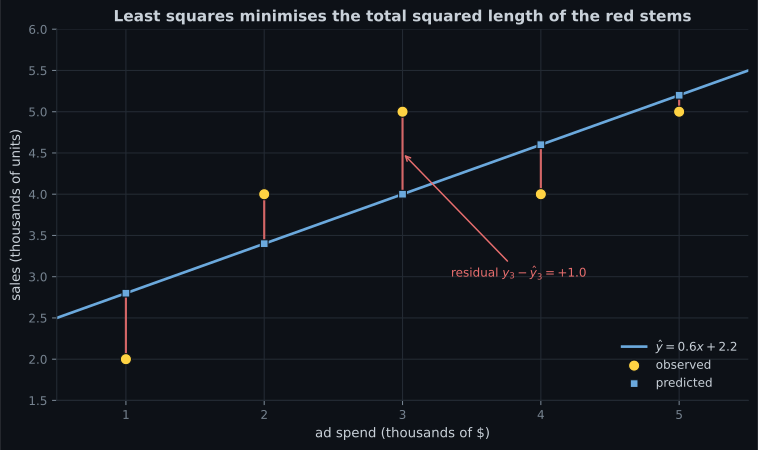
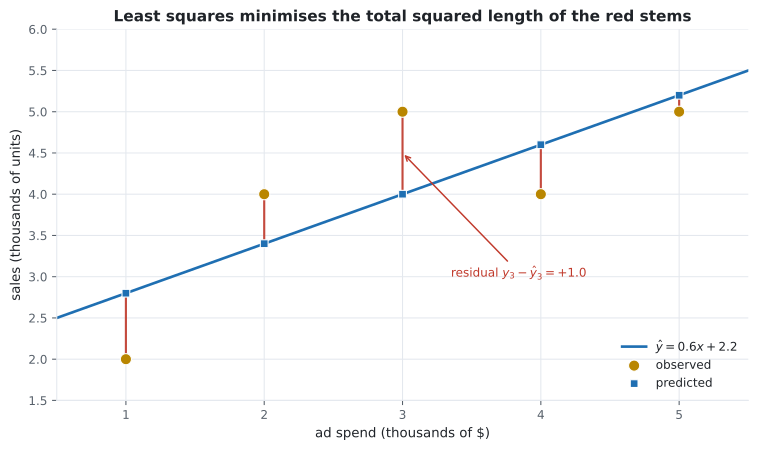
So the fitted line is $\hat{y} = 0.6x + 2.2$. Every extra thousand dollars of spend buys 600 more units of sales.

Step 4 — predictions and residuals.

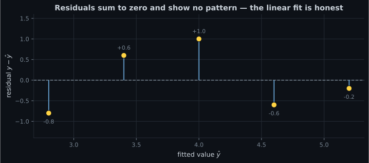
The residuals sum to exactly zero. That is not luck — it is the first normal equation, $\sum e_i = 0$, which is what fixing $b = \bar{y} - w\bar{x}$ guarantees.

Step 5 — the error numbers.

Step 6 — how much did we explain? Compare against the dumbest possible model, which always predicts $\bar{y} = 4$:

The line removes 60% of the variance that predicting the mean would have left. Metrics R-Squared and Adjusted R-Squared takes that number apart properly.

figureThe fitted line and its five residualsmatplotlib

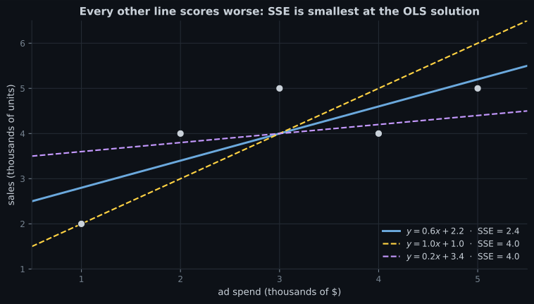
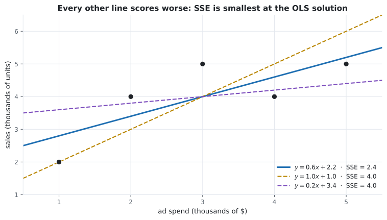
Why no other line beats it

Two plausible alternatives, scored on the same five points:

figureThree candidate lines, three SSE scoresmatplotlib

See it move

Below, the line starts flat and walks toward the least-squares solution by repeatedly nudging $w$ and $b$ downhill. The closed-form answer and the iterative one land in the same place; the iterative route is the one that keeps working when there are a million features.

From scratch

The two formulas, transcribed directly. No optimiser, no library model:

import numpy as np
 
 
def fit_simple_linear(x, y):
    """Return (w, b) for the least-squares line through 1-D data."""
    x, y = np.asarray(x, dtype=float), np.asarray(y, dtype=float)
    x_mean, y_mean = x.mean(), y.mean()
 
    # w = Cov(x, y) / Var(x), written out as the two sums from the derivation
    numerator = ((x - x_mean) * (y - y_mean)).sum()
    denominator = ((x - x_mean) ** 2).sum()
    if denominator == 0:
        raise ValueError("x has zero variance — no line is determined")
 
    w = numerator / denominator
    b = y_mean - w * x_mean
    return w, b
 
 
x = [1, 2, 3, 4, 5]
y = [2, 4, 5, 4, 5]
 
w, b = fit_simple_linear(x, y)
pred = w * np.array(x) + b
resid = np.array(y) - pred
 
print(f"w = {w}")                    # w = 0.6
print(f"b = {b}")                    # b = 2.2
print(f"residuals = {resid}")        # residuals = [-0.8  0.6  1.  -0.6 -0.2]
print(f"SSE = {(resid ** 2).sum()}") # SSE = 2.4

import numpy as np
 
 
def fit_simple_linear(x, y):
    """Return (w, b) for the least-squares line through 1-D data."""
    x, y = np.asarray(x, dtype=float), np.asarray(y, dtype=float)
    x_mean, y_mean = x.mean(), y.mean()
 
    # w = Cov(x, y) / Var(x), written out as the two sums from the derivation
    numerator = ((x - x_mean) * (y - y_mean)).sum()
    denominator = ((x - x_mean) ** 2).sum()
    if denominator == 0:
        raise ValueError("x has zero variance — no line is determined")
 
    w = numerator / denominator
    b = y_mean - w * x_mean
    return w, b
 
 
x = [1, 2, 3, 4, 5]
y = [2, 4, 5, 4, 5]
 
w, b = fit_simple_linear(x, y)
pred = w * np.array(x) + b
resid = np.array(y) - pred
 
print(f"w = {w}")                    # w = 0.6
print(f"b = {b}")                    # b = 2.2
print(f"residuals = {resid}")        # residuals = [-0.8  0.6  1.  -0.6 -0.2]
print(f"SSE = {(resid ** 2).sum()}") # SSE = 2.4

Every number matches the hand calculation, which is the point of doing both.

With scikit-learn

The same fit through the estimator API. Note the reshape(-1, 1)reshape(-1, 1) — scikit-learn always wants XX two-dimensional, one row per sample and one column per feature, even when there is only one feature:

import numpy as np
from sklearn.linear_model import LinearRegression
from sklearn.metrics import mean_squared_error, r2_score
 
X = np.array([1, 2, 3, 4, 5]).reshape(-1, 1)   # (5, 1) — 5 samples, 1 feature
y = np.array([2, 4, 5, 4, 5])
 
model = LinearRegression()
model.fit(X, y)
 
print(f"w = {model.coef_[0]:.4f}")        # w = 0.6000
print(f"b = {model.intercept_:.4f}")      # b = 2.2000
 
pred = model.predict(X)
print(f"MSE = {mean_squared_error(y, pred):.4f}")  # MSE = 0.4800
print(f"R^2 = {r2_score(y, pred):.4f}")            # R^2 = 0.6000
 
# Predicting for a new spend level
print(f"x=6 -> {model.predict([[6]])[0]:.2f}")     # x=6 -> 5.80

import numpy as np
from sklearn.linear_model import LinearRegression
from sklearn.metrics import mean_squared_error, r2_score
 
X = np.array([1, 2, 3, 4, 5]).reshape(-1, 1)   # (5, 1) — 5 samples, 1 feature
y = np.array([2, 4, 5, 4, 5])
 
model = LinearRegression()
model.fit(X, y)
 
print(f"w = {model.coef_[0]:.4f}")        # w = 0.6000
print(f"b = {model.intercept_:.4f}")      # b = 2.2000
 
pred = model.predict(X)
print(f"MSE = {mean_squared_error(y, pred):.4f}")  # MSE = 0.4800
print(f"R^2 = {r2_score(y, pred):.4f}")            # R^2 = 0.6000
 
# Predicting for a new spend level
print(f"x=6 -> {model.predict([[6]])[0]:.2f}")     # x=6 -> 5.80

On real data

Five tidy points are a teaching device. Here is the same estimator on 442 real patients from the load_diabetesload_diabetes dataset, predicting one-year disease progression from body mass index alone:

from sklearn.datasets import load_diabetes
from sklearn.linear_model import LinearRegression
 
data = load_diabetes()
bmi = data.data[:, 2].reshape(-1, 1)   # column 2 is the standardised BMI
y = data.target
 
model = LinearRegression().fit(bmi, y)
 
print(f"w   = {model.coef_[0]:.2f}")        # w   = 949.44
print(f"b   = {model.intercept_:.2f}")      # b   = 152.13
print(f"R^2 = {model.score(bmi, y):.4f}")   # R^2 = 0.3439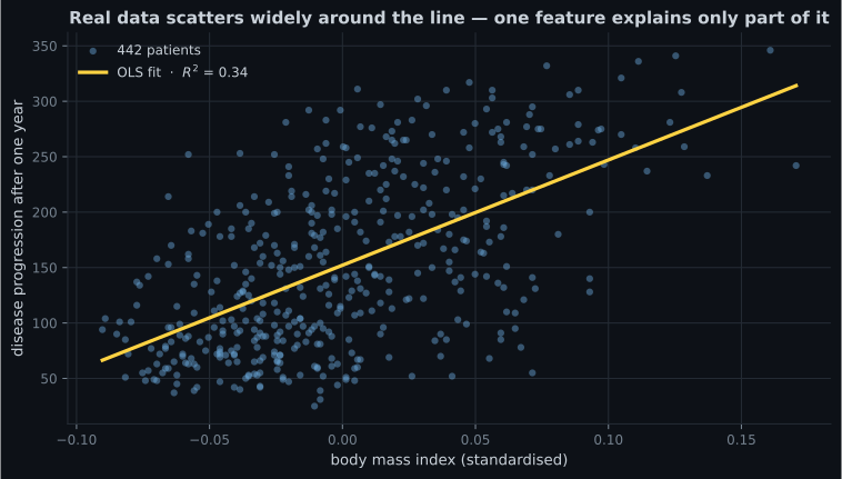

from sklearn.datasets import load_diabetes
from sklearn.linear_model import LinearRegression
 
data = load_diabetes()
bmi = data.data[:, 2].reshape(-1, 1)   # column 2 is the standardised BMI
y = data.target
 
model = LinearRegression().fit(bmi, y)
 
print(f"w   = {model.coef_[0]:.2f}")        # w   = 949.44
print(f"b   = {model.intercept_:.2f}")      # b   = 152.13
print(f"R^2 = {model.score(bmi, y):.4f}")   # R^2 = 0.3439

figureOne feature on 442 real patientsmatplotlib

Reading the plot

Three things to take from that figure, in the order you should check them:

1. The direction is real. The cloud tilts upward consistently, not just at the edges. A positive slope here is a genuine signal, not an artefact of two outliers.
2. The spread grows with $x$. Points on the right scatter further from the line than points on the left. That is heteroscedasticity — it does not bias the slope, but it does make the usual confidence intervals too optimistic.
3. $R^2 = 0.34$ is not a failure. For a single biological predictor it is a strong result. It is a signal that more features would help, which is exactly what the next page does.

The residual plot is where you confirm all three at a glance. For the five-point example it looks like this — no curve, no fan, no runaway point:

figureResiduals versus fitted valuesmatplotlib

The four assumptions

Least squares is always computable. It is only trustworthy when these hold:

Only linearity affects the point predictions. The other three affect how much you should believe the confidence intervals around them.

Pitfalls

Compare

🧪 Try It Yourself

Exercise 1 – Compute the slope by hand

Exercise 2 – Push the line through the centroid

Exercise 3 – Residuals must sum to zero

Exercise 4 – Reproduce it with scikit-learn

Exercise 5 – Watch one outlier wreck the fit

Recap

• The model is $\hat{y} = wx + b$; the loss is $\sum (y_i - \hat{y}_i)^2$.
• Setting both partial derivatives to zero gives $w = \operatorname{Cov}(x,y)/\operatorname{Var}(x)$ and $b = \bar{y} - w\bar{x}$ — no iteration required.
• The fitted line always passes through $(\bar{x}, \bar{y})$, and residuals always sum to zero.
• $R^2$ compares your SSE against the SSE of predicting the mean; 0.60 on the worked example, 0.34 on real diabetes data.
• Squaring the errors buys differentiability and a closed form, and costs robustness to outliers.
• Check linearity and equal variance in the residual plot before believing anything else.

Exercise 6 – Check the three identities a least-squares fit must satisfy

Next

Continue to Multiple Linear Regression — the same idea with many features at once, where the two scalar formulas become one matrix equation and interpreting a coefficient gets considerably subtler.