Autoencoders

An autoencoder learns to copy its input through a bottleneck. The encoder compresses, the decoder reconstructs, and the loss is how badly the copy came out. Nothing labels the data, so it is unsupervised — and the compression is supposed to be the useful part.

There is an exact baseline for that claim, and it is rarely run. A linear autoencoder trained with squared error learns the same subspace as PCA. So a nonlinear autoencoder has to beat PCA at the same number of components, or its training time bought nothing.

Bottleneck	Autoencoder MSE	PCA MSE	Autoencoder vs PCA
2	0.0456	0.0542	+16.0%
8	0.0254	0.0368	+31.1%
32	0.0155	0.0159	+2.3%
128	0.0114	0.0035	−229.0%

The nonlinearity pays at a tight bottleneck and loses badly at a loose one — where PCA reconstructs more than three times better than the trained network.

What you’ll learn

• The encoder–bottleneck–decoder shape, and why the bottleneck is the whole design.
• Why PCA is the correct baseline, and where the autoencoder beats it.
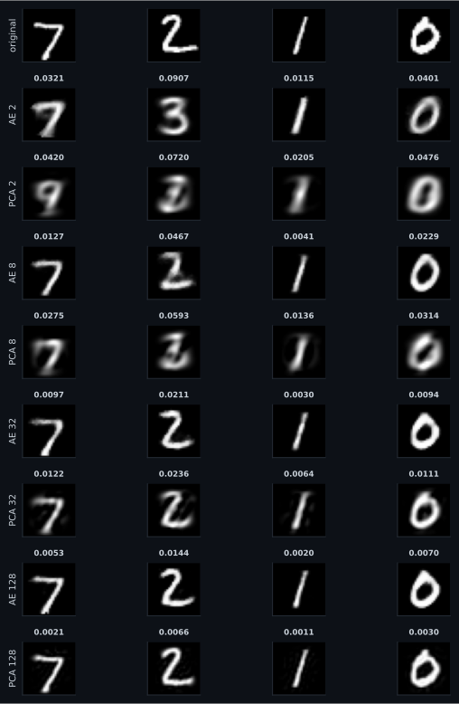
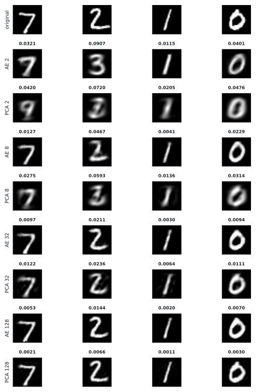
• What reconstructions actually look like at 2, 8, 32 and 128 dimensions.
• Why a 128-dimensional autoencoder lost to a closed-form method.
• Denoising autoencoders, and the 3×3 blur baseline that halves the error for free.
• Why none of this makes an autoencoder a generative model.

The shape

Encoder, bottleneck, decoder

inputs = keras.layers.Input((784,))
x = keras.layers.Dense(256, activation="relu")(inputs)
x = keras.layers.Dense(64, activation="relu")(x)
code = keras.layers.Dense(bottleneck, activation="relu", name="code")(x)   # <- the whole point
x = keras.layers.Dense(64, activation="relu")(code)
x = keras.layers.Dense(256, activation="relu")(x)
outputs = keras.layers.Dense(784, activation="sigmoid")(inputs)
model.compile("adam", "mse")            # the target IS the input

The only thing stopping the network learning the identity function is that the code layer is narrower than the input. Everything interesting follows from that constraint: with a wide enough bottleneck the task is trivial and the representation is useless.

PCA is the baseline

$$\min_{W, W'} \; \lVert X - X W W' \rVert_F^2$$

With linear activations and squared error, that is exactly the problem PCA solves in closed form. Adding nonlinearity means the autoencoder can represent curved manifolds PCA cannot — but it also has to find them by gradient descent.

figure MNIST, 12,000 images, 20 epochs matplotlib

Two regimes, and the crossover is the interesting part. At a tight bottleneck the nonlinearity earns its keep: 8 components of PCA keep 44.7% of the variance while the autoencoder's 8 numbers reconstruct 31.1% better. At 128 components PCA keeps 93.9% of the variance and reconstructs 3.3x better than the network — because at that width the problem is nearly linear, PCA solves it exactly, and gradient descent on 452,112 parameters simply does not get as close in 20 epochs.

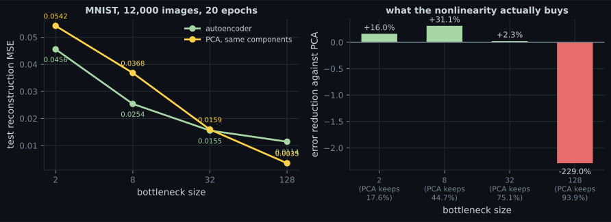
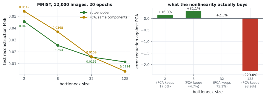
That −229.0% deserves stating plainly: the closed-form method beat the neural network by a factor of 3.3. Not because autoencoders are bad, but because at 128 dimensions there is little curvature left to exploit, PCA is optimal for squared error, and an optimiser working on a non-convex objective with a fixed budget lands somewhere worse.

figure The same four digits at every bottleneck matplotlib

At 2 dimensions neither method reconstructs the digit — they reconstruct the average digit that lands in that region of the code space, which is why the numbers are often wrong rather than merely blurry. The 128-dimensional rows are where the numeric result becomes visible: the PCA reconstructions have sharper strokes because they are the exact least-squares projection, while the autoencoder's are smoothed by an optimiser that stopped early.

Denoising

Change one thing — feed corrupted input and ask for the clean image — and the autoencoder stops learning compression and starts learning the data distribution’s structure.

The only change is the training pair

model.fit(noisy_train, clean_train, ...)      # input != target

Method	MSE against the clean image
do nothing (the noisy input)	0.0798
3×3 blur	0.0446
denoising autoencoder	0.0237

figure Gaussian noise, standard deviation 0.4 matplotlib

The blur is the baseline that makes the autoencoder's number meaningful. Averaging nine neighbouring pixels removes almost half the error for free, with no training and no parameters, because the noise is independent per pixel and the signal is not. The autoencoder halves the error again — that remaining factor of 1.9 is what learning the digit distribution actually bought.

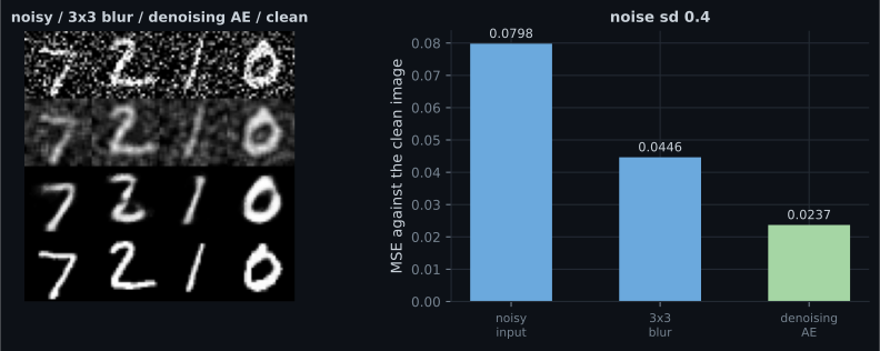
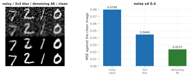
Without the blur baseline, “0.0237 MSE” is unanchored. With it, the claim becomes specific: the network is worth 1.9× a three-line convolution, on this noise level.

What an autoencoder is not

An autoencoder is not a generative model, and the reason is worth being precise about. Nothing in the training objective constrains what the code space looks like — only that the decoder can invert the encoder on points the encoder actually produces. So:

• Sampling a random code vector and decoding it produces nothing meaningful, because random points are nowhere near the region the encoder uses.
• With a ReLU code layer, most of the space is unreachable by construction — codes are non-negative.
• The code distribution has no reason to be smooth or connected, so interpolating between two codes can pass through empty regions.

Fixing exactly this — by forcing the code distribution towards a known prior — is what the next page is about, and it is the difference between compression and generation.

diagram Diagram mermaid

  flowchart LR
  A["input 784"] --> B["Dense 256"]
  B --> C["Dense 64"]
  C --> D["code
2 / 8 / 32 / 128"]
  D --> E["Dense 64"]
  E --> F["Dense 256"]
  F --> G["output 784"]
  G -.->|"MSE against the input"| A
  D -.->|"tight: nonlinearity wins
+31.1% over PCA"| H["compression"]
  D -.->|"loose: PCA wins
-229.0%"| H
  D -.->|"no constraint on the
shape of this space"| I["not a generative model"]

sketch What a bottleneck can carry p5.js Pause Restart

Drag the bottleneck size. The bar shows how much of MNIST's variance PCA keeps at that many components, with the measured autoencoder and PCA errors alongside.

sketch The measured table, ranked p5.js Pause Restart

Click a column to rank every row by it. The bars are that column's values and the highest and lowest are computed from the numbers, not written in.

Pitfalls

• Not running PCA. It is two lines, needs no training, and beat the autoencoder by 3.3× at 128 components.
• Claiming an autoencoder “learns features” without a downstream test. Reconstruction error measures reconstruction; use a linear probe if you care about the features.
• Using a wide bottleneck. At 128 of 784 dimensions the task is nearly linear and the representation is barely compressed.
• Sampling random codes and expecting digits. Nothing constrains the code distribution; with a ReLU code layer most of the space is unreachable.
• Reporting a denoiser without a blur baseline. A 3×3 average removed 44% of the error for free.
• Comparing MSE across noise levels or datasets. The number is only meaningful against a baseline on the same data.
• Expecting sharp reconstructions from squared error. MSE’s optimum is the conditional mean, which is why every reconstruction on this page is smooth.

Recap

• An autoencoder minimises reconstruction error through a bottleneck; the bottleneck is the only thing preventing the identity function.
• A linear autoencoder with squared error is PCA, so PCA at the same component count is the baseline.
• Measured: autoencoder better by 16.0% at 2 components and 31.1% at 8; PCA better by 3.3× at 128.
• PCA’s explained variance at those widths: 17.6%, 44.7%, 75.1%, 93.9%.
• Denoising: noisy input 0.0798, 3×3 blur 0.0446, denoising autoencoder 0.0237.
• An autoencoder is not generative — nothing shapes the code distribution, which is exactly what a VAE adds.

Next

Add one constraint — that the code distribution match a known prior — and the same architecture becomes able to generate: Variational Autoencoders (VAE).

pch.quizTag pch.quizDefaultTitle

1. Why is PCA the right baseline for an autoencoder?

   A Because it is faster B Because a linear autoencoder trained with squared error learns the same subspace as PCA — so the nonlinear version must beat PCA at the same component count to have earned anything C Because PCA also uses gradient descent D Because PCA works only on images
   pch.quizShowAnswer

   B — Because a linear autoencoder trained with squared error learns the same subspace as PCA — so the nonlinear version must beat PCA at the same component count to have earned anything — Measured: the autoencoder won by 31.1% at 8 components and lost by a factor of 3.3 at 128.

2. At a 128-dimensional bottleneck, PCA reached MSE 0.0035 against the autoencoder's 0.0114. What explains that?

   A The autoencoder was implemented incorrectly B At that width the problem is nearly linear — PCA keeps 93.9% of the variance and solves least squares exactly, while gradient descent on 452,112 parameters lands somewhere worse in 20 epochs C PCA is always better than autoencoders D MSE is the wrong metric for PCA
   pch.quizShowAnswer

   B — At that width the problem is nearly linear — PCA keeps 93.9% of the variance and solves least squares exactly, while gradient descent on 452,112 parameters lands somewhere worse in 20 epochs — The nonlinearity only pays where there is curvature to exploit, which is at a tight bottleneck — +16.0% at 2 dimensions and +31.1% at 8.

3. A denoising autoencoder scored MSE 0.0237 against the clean images. Why is that number not interpretable on its own?

   A Because MSE is not a valid metric for images B Because a 3x3 average blur — no training, no parameters — already scores 0.0446 against the noisy input's 0.0798, so the network's real contribution is a further factor of 1.9 C Because the noise level was too low D Because denoising is not a learning problem
   pch.quizShowAnswer

   B — Because a 3x3 average blur — no training, no parameters — already scores 0.0446 against the noisy input's 0.0798, so the network's real contribution is a further factor of 1.9 — Independent per-pixel noise is exactly what local averaging removes, so the blur is the baseline that anchors the claim.

4. Why can't you generate new digits by sampling a random code vector and decoding it?

   A Because the decoder is not invertible B Because nothing in the loss constrains the code distribution — random points are far from the region the encoder actually produces, and with a ReLU code layer most of the space is unreachable C Because the bottleneck is too small D Because MSE cannot generate images
   pch.quizShowAnswer

   B — Because nothing in the loss constrains the code distribution — random points are far from the region the encoder actually produces, and with a ReLU code layer most of the space is unreachable — Forcing the code distribution towards a known prior is precisely the change a VAE makes, and it is the difference between compression and generation.

5. At a 2-dimensional bottleneck the reconstructions often show the wrong digit rather than a blurry right one. Why?

   A The model is undertrained B Two numbers cannot identify a digit, so the decoder outputs the average image for that region of the code space — and the average of several digit classes is a different digit C The sigmoid output saturates D MNIST digits are ambiguous at low resolution
   pch.quizShowAnswer

   B — Two numbers cannot identify a digit, so the decoder outputs the average image for that region of the code space — and the average of several digit classes is a different digit — Squared error's optimum is the conditional mean, so a bottleneck too tight to disambiguate produces a mean over classes.

🧪 Try It Yourself

pch.exerciseTag pch.exerciseTitle

pch.exerciseTag pch.exerciseTitle

pch.exerciseTag pch.exerciseTitle

pch.exerciseTag pch.exerciseTitle

pch.exerciseTag pch.exerciseTitle