Determinant and Trace

Before factoring a matrix it helps to have a couple of numbers that summarise it. This page gives two: the determinant, which is a signed volume and decides invertibility, and the trace, which is the sum of the diagonal.

Both are cheap, both are single numbers, and — the property that makes them worth defining — both are invariant under a change of basis. They describe the linear mapping, not the particular matrix you happened to write down for it.

What you’ll learn

• The determinant for $n = 1, 2, 3$, the Laplace expansion for general $n$, and the triangular shortcut.
• Why $\det\mathbf{A} \neq 0$, invertibility, and full rank are the same condition (Theorems 4.1 and 4.3).
• The determinant as a signed volume, verified on the book’s Example 4.2 where the answer is $186$.
• The seven properties of the determinant, each measured.
• The trace, its four defining properties, and the cyclic-permutation identity that makes it useful.
• Equation 4.21: the trace of a linear mapping is basis independent, measured over two thousand random changes of basis.
• The characteristic polynomial, whose constant term is the determinant and whose next coefficient is the trace.

Intuition: how much does this map stretch space?

Feed the unit square through a $2\times2$ matrix and you get a parallelogram. Its area is $\lvert\det\mathbf{A}\rvert$. Feed the unit cube through a $3\times3$ matrix and you get a parallelepiped, whose volume is again $\lvert\det\mathbf{A}\rvert$.

That one sentence explains most of the determinant’s behaviour before any algebra:

• $\det = 0$ means the volume collapsed, so the map squashed space into a lower dimension, so it threw information away, so it cannot be inverted.
• $\det(\mathbf{A}\mathbf{B}) = \det\mathbf{A}\det\mathbf{B}$ because applying two maps in sequence multiplies their stretch factors.
• $\det(\lambda\mathbf{A}) = \lambda^n\det\mathbf{A}$ because scaling all $n$ edges of a box by $\lambda$ scales its volume by $\lambda^n$.
• The sign records orientation: whether the map preserved handedness or mirrored it.

The trace has no such picture in general — it is a sum of diagonal entries, which are basis-dependent quantities. What makes it meaningful is that the sum is not.

diagram Diagram mermaid

  flowchart TD
  A["a square matrix A"]
  A --> DET["det A = signed volume
Eq 4.1"]
  A --> TR["tr A = sum of the diagonal
Eq 4.18"]
  DET --> INV["det A ≠ 0 ⟺ invertible
⟺ full rank
Thm 4.1, 4.3"]
  DET --> PROD["det(AB) = det A · det B
det(λA) = λⁿ det A"]
  TR --> CYC["tr(AKL) = tr(KLA)
invariant under cyclic permutation
Eq 4.19"]
  DET --> BASIS["both survive A ↦ S⁻¹AS
Eq 4.21"]
  TR --> BASIS
  BASIS --> MAP["so they describe the MAPPING,
not the matrix"]
  DET --> CP["characteristic polynomial
p(λ) = det(A − λI)
Def 4.5"]
  TR --> CP
  CP --> EIG["→ eigenvalues, §4.2"]

The math

Small determinants

Equations 4.5, 4.6 and 4.7

$$n = 1: \quad \det\mathbf{A} = a_{11}$$$$n = 2: \quad \det\mathbf{A} = \begin{vmatrix} a_{11} & a_{12}\\ a_{21} & a_{22}\end{vmatrix} = a_{11}a_{22} - a_{12}a_{21}$$$$n = 3 \ \text{(Sarrus' rule)}: \quad \det\mathbf{A} = a_{11}a_{22}a_{33} + a_{21}a_{32}a_{13} + a_{31}a_{12}a_{23} - a_{31}a_{22}a_{13} - a_{11}a_{32}a_{23} - a_{21}a_{12}a_{33}$$

The $2\times2$ case is not arbitrary. Example 4.1 derives it: the inverse of a $2\times2$ matrix is

$$\mathbf{A}^{-1} = \frac{1}{a_{11}a_{22} - a_{12}a_{21}}\begin{bmatrix} a_{22} & -a_{12}\\ -a_{21} & a_{11}\end{bmatrix}$$

so the matrix is invertible exactly when that denominator is nonzero. The determinant is not a formula someone invented; it is the quantity that has to be nonzero for the inverse to exist, extracted and named.

Theorem 4.1 and Theorem 4.3

For any square $\mathbf{A} \in \mathbb{R}^{n\times n}$:

$$\mathbf{A} \text{ is invertible} \iff \det\mathbf{A} \neq 0 \iff \mathrm{rk}(\mathbf{A}) = n$$

Triangular matrices, and the fast route

Equation 4.8

A matrix $\mathbf{T}$ is upper triangular if $T_{ij} = 0$ for $i > j$, and lower triangular if it is zero above the diagonal. For any triangular $\mathbf{T} \in \mathbb{R}^{n\times n}$,

$$\det\mathbf{T} = \prod_{i=1}^{n} T_{ii}$$

This is the whole practical algorithm. Gaussian elimination brings a matrix to triangular form using only operations whose effect on the determinant is known — adding a multiple of one row to another changes nothing, scaling a row by $\lambda$ multiplies by $\lambda$, swapping two rows flips the sign — so you eliminate, multiply the diagonal, and correct for what you did.

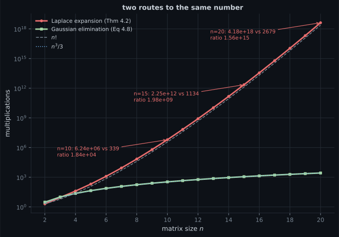
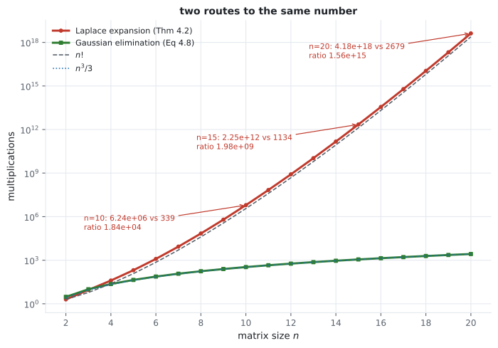
The Laplace expansion

Theorem 4.2 — Laplace expansion

For $\mathbf{A} \in \mathbb{R}^{n\times n}$ and any $j = 1,\dots,n$:

along column $j$:

$$\det\mathbf{A} = \sum_{k=1}^{n} (-1)^{k+j} a_{kj} \det\mathbf{A}_{k,j}$$

along row $j$:

$$\det\mathbf{A} = \sum_{k=1}^{n} (-1)^{k+j} a_{jk} \det\mathbf{A}_{j,k}$$

where $\mathbf{A}_{k,j} \in \mathbb{R}^{(n-1)\times(n-1)}$ is $\mathbf{A}$ with row $k$ and column $j$ deleted. $\det\mathbf{A}_{k,j}$ is a minor and $(-1)^{k+j}\det\mathbf{A}_{k,j}$ a cofactor.

The recursion is correct and unusable. Expanding an $n\times n$ determinant needs $n$ sub-determinants of size $n-1$, so the count satisfies $L(n) = n\,L(n-1) + n$ — which grows like $n!$. Measured against Gaussian elimination’s $n^3/3$:

$n$	Laplace multiplications	Gaussian elimination	ratio
3	$9$	$10$	$0.9$
5	$205$	$44$	$4.7$
10	$6.24\times10^{6}$	$339$	$1.8\times10^{4}$
15	$2.25\times10^{12}$	$1134$	$2.0\times10^{9}$
20	$4.18\times10^{18}$	$2679$	$1.6\times10^{15}$

At $n = 3$ the recursion is actually cheaper, which is why hand calculation uses it and why it feels reasonable. By $n = 20$ it is fifteen orders of magnitude worse.

The seven properties

For $\mathbf{A} \in \mathbb{R}^{n\times n}$:

property	statement	measured gap
multiplicative	$\det(\mathbf{A}\mathbf{B}) = \det\mathbf{A}\,\det\mathbf{B}$	$5.3\times10^{-15}$
transpose-invariant	$\det\mathbf{A} = \det\mathbf{A}^\top$	$2.7\times10^{-15}$
inverse	$\det(\mathbf{A}^{-1}) = \dfrac{1}{\det\mathbf{A}}$	$5.6\times10^{-17}$
similarity-invariant	similar matrices have the same determinant	see the figure
row addition	adding a multiple of a row to another leaves $\det$ unchanged	$3.6\times10^{-15}$
row scaling	scaling a row by $\lambda$ scales $\det$ by $\lambda$; so $\det(\lambda\mathbf{A}) = \lambda^n\det\mathbf{A}$	exact ratio $4.0$ and $\lambda^5$
row swap	swapping two rows flips the sign	exact ratio $-1$

All measured on random $5\times5$ matrices. The last three are what license Gaussian elimination as a determinant algorithm.

The trace

Definition 4.4 and Equation 4.18

$$\mathrm{tr}(\mathbf{A}) := \sum_{i=1}^{n} a_{ii}$$

with the properties

$$\mathrm{tr}(\mathbf{A}+\mathbf{B}) = \mathrm{tr}(\mathbf{A}) + \mathrm{tr}(\mathbf{B}), \qquad \mathrm{tr}(\alpha\mathbf{A}) = \alpha\,\mathrm{tr}(\mathbf{A}),$$$$\mathrm{tr}(\mathbf{I}_n) = n, \qquad \mathrm{tr}(\mathbf{A}\mathbf{B}) = \mathrm{tr}(\mathbf{B}\mathbf{A}) \text{ for } \mathbf{A}\in\mathbb{R}^{n\times k},\ \mathbf{B}\in\mathbb{R}^{k\times n}$$

The book notes that only one function satisfies all four together — the trace.

The fourth property is stranger than it looks: $\mathbf{A}\mathbf{B}$ is $n\times n$ and $\mathbf{B}\mathbf{A}$ is $k\times k$, so those are matrices of different sizes with the same trace. Measured on a $4\times6$ times a $6\times4$: both traces come to $-0.1133701535$, from a $4\times4$ and a $6\times6$ respectively.

It generalises to invariance under cyclic permutation (Equation 4.19):

$$\mathrm{tr}(\mathbf{A}\mathbf{K}\mathbf{L}) = \mathrm{tr}(\mathbf{K}\mathbf{L}\mathbf{A})$$

and specialises, for vectors, to Equation 4.20:

$$\mathrm{tr}(\mathbf{x}\mathbf{y}^\top) = \mathrm{tr}(\mathbf{y}^\top\mathbf{x}) = \mathbf{y}^\top\mathbf{x} \in \mathbb{R}$$

That last identity is the one you will actually use. It turns the trace of an $n\times n$ outer product into a single dot product, and it is how every “trace trick” derivation in machine learning starts.

Basis independence

Equation 4.21

For an invertible $\mathbf{S}$,

$$\mathrm{tr}(\mathbf{S}^{-1}\mathbf{A}\mathbf{S}) \overset{(4.19)}{=} \mathrm{tr}(\mathbf{A}\mathbf{S}\mathbf{S}^{-1}) = \mathrm{tr}(\mathbf{A})$$

So while the matrix representing a linear mapping $\Phi$ depends on the basis, the trace of $\Phi$ does not. The same holds for the determinant, by the multiplicative property.

The proof is one application of cyclic invariance. This is the property that promotes both quantities from “facts about a matrix” to “facts about a mapping”, and the reason they belong in the same section as the eigenvalues, which share it.

The characteristic polynomial

Definition 4.5 — Characteristic polynomial

For $\lambda \in \mathbb{R}$ and a square $\mathbf{A} \in \mathbb{R}^{n\times n}$,

$$p_{\mathbf{A}}(\lambda) := \det(\mathbf{A} - \lambda\mathbf{I}) = c_0 + c_1\lambda + c_2\lambda^2 + \dots + c_{n-1}\lambda^{n-1} + (-1)^n\lambda^n$$

In particular

$$c_0 = \det(\mathbf{A}), \qquad c_{n-1} = (-1)^{n-1}\mathrm{tr}(\mathbf{A})$$

Set $\lambda = 0$ and the first identity is immediate. The second takes a little more work and is worth knowing because it means the determinant and the trace are two coefficients of the same polynomial — the bottom one and the top-but-one. §4.2 will show that the polynomial’s roots are the eigenvalues, at which point $\det = \prod\lambda_i$ and $\mathrm{tr} = \sum\lambda_i$ follow as Theorems 4.16 and 4.17.

From the book

Section 4.1. Equation 4.1 defines the notation, with a margin warning that $\lvert\mathbf{A}\rvert$ must not be confused with an absolute value. Example 4.1 derives the $2\times2$ case from the inverse (Equations 4.2 to 4.4); Theorem 4.1 is the invertibility criterion. Equations 4.5 to 4.7 give $n = 1, 2, 3$ with Sarrus’ rule; Equation 4.8 the triangular product. Example 4.2 is the volume interpretation, with Figures 4.2 and 4.3 and the vectors of Equation 4.9 giving $V = 186$ in Equation 4.11. Theorem 4.2 is the Laplace expansion (Equations 4.12 and 4.13) with Example 4.3 (Equations 4.14 to 4.17). The seven properties follow, then Theorem 4.3 tying $\det \neq 0$ to full rank. The book then remarks that contemporary numerical methods superseded the explicit calculation of the determinant. Definition 4.4 and Equation 4.18 give the trace, Equations 4.19 and 4.20 its permutation identities, Equation 4.21 basis independence, and Definition 4.5 with Equations 4.22 to 4.24 the characteristic polynomial.

Worked example by hand

Example 4.3 — Laplace expansion

$$\mathbf{A} = \begin{bmatrix} 1 & 2 & 3\\ 3 & 1 & 2\\ 0 & 0 & 1\end{bmatrix}$$

Expand along the first row, so $j = 1$ in Equation 4.13:

$$\begin{vmatrix} 1 & 2 & 3\\ 3 & 1 & 2\\ 0 & 0 & 1\end{vmatrix} = (-1)^{1+1}\cdot 1 \begin{vmatrix} 1 & 2\\ 0 & 1\end{vmatrix} + (-1)^{1+2}\cdot 2 \begin{vmatrix} 3 & 2\\ 0 & 1\end{vmatrix} + (-1)^{1+3}\cdot 3 \begin{vmatrix} 3 & 1\\ 0 & 0\end{vmatrix}$$

Each $2\times2$ by Equation 4.6:

minor	working	value
$\begin{vmatrix}1&2\\0&1\end{vmatrix}$	$1(1) - 2(0)$	$1$
$\begin{vmatrix}3&2\\0&1\end{vmatrix}$	$3(1) - 2(0)$	$3$
$\begin{vmatrix}3&1\\0&0\end{vmatrix}$	$3(0) - 1(0)$	$0$

$$\det\mathbf{A} = 1(1) - 2(3) + 3(0) = 1 - 6 = -5$$

Cross-check with Sarrus’ rule (Equation 4.17):

$$1\cdot1\cdot1 + 3\cdot0\cdot3 + 0\cdot2\cdot2 - 0\cdot1\cdot3 - 1\cdot0\cdot2 - 3\cdot2\cdot1 = 1 - 6 = -5$$

Both routes give $-5$, matching Equations 4.16 and 4.17.

A third route is faster than either. The third row is $(0, 0, 1)$, so expanding along that row leaves one term:

$$\det\mathbf{A} = (-1)^{3+3}\cdot 1 \begin{vmatrix}1&2\\3&1\end{vmatrix} = 1 - 6 = -5$$

Laplace lets you choose the row or column, and choosing the one with the most zeros is free.

Example 4.2 — volume

$$\mathbf{r} = \begin{bmatrix}2\\0\\-8\end{bmatrix}, \quad \mathbf{g} = \begin{bmatrix}6\\1\\0\end{bmatrix}, \quad \mathbf{b} = \begin{bmatrix}1\\4\\-1\end{bmatrix} \qquad\Longrightarrow\qquad \mathbf{A} = [\mathbf{r}, \mathbf{g}, \mathbf{b}] = \begin{bmatrix}2&6&1\\0&1&4\\-8&0&-1\end{bmatrix}$$

Sarrus:

$$2(1)(-1) + 0(0)(1) + (-8)(6)(4) - (-8)(1)(1) - 2(0)(4) - 0(6)(-1) = -2 + 0 - 192 + 8 - 0 - 0 = -186$$

so $V = \lvert\det\mathbf{A}\rvert = 186$, which is Equation 4.11. The determinant itself is $-186$: the three vectors form a left-handed frame.

determinants_worked.py

import numpy as np
 
# Example 4.3
A = np.array([[1.0, 2.0, 3.0], [3.0, 1.0, 2.0], [0.0, 0.0, 1.0]])
print("det:", float(np.linalg.det(A)))
print("Laplace, first row: 1*(1) - 2*(3) + 3*(0) =", 1 * 1 - 2 * 3 + 3 * 0)
print("Laplace, third row: 1*(1*1 - 2*3)         =", 1 * (1 * 1 - 2 * 3))
 
# Example 4.2
r, g, b = np.array([2.0, 0, -8]), np.array([6.0, 1, 0]), np.array([1.0, 4, -1])
V = np.stack([r, g, b], axis=1)
print("det [r, g, b] =", float(np.linalg.det(V)), " volume =", abs(float(np.linalg.det(V))))
 
# The seven properties, measured on random 5x5 matrices.
rng = np.random.default_rng(11)
X, Y = rng.normal(size=(5, 5)), rng.normal(size=(5, 5))
dX = float(np.linalg.det(X))
print("det(XY) - det(X)det(Y):", f"{abs(float(np.linalg.det(X @ Y)) - dX * float(np.linalg.det(Y))):.3e}")
print("det(X)  - det(X^T)    :", f"{abs(dX - float(np.linalg.det(X.T))):.3e}")
print("det(inv X) - 1/det(X) :", f"{abs(float(np.linalg.det(np.linalg.inv(X))) - 1 / dX):.3e}")
print("det(2.7 X)/det(X) =", round(float(np.linalg.det(2.7 * X)) / dX, 6), " 2.7^5 =", round(2.7 ** 5, 6))
 
Z = X.copy(); Z[1] += 3.4 * Z[0]
print("row addition changes det by:", f"{abs(float(np.linalg.det(Z)) - dX):.3e}")
Z = X.copy(); Z[[0, 2]] = Z[[2, 0]]
print("row swap det ratio:", round(float(np.linalg.det(Z)) / dX, 12))
Z = X.copy(); Z[2] *= 4.0
print("row scaling det ratio:", round(float(np.linalg.det(Z)) / dX, 10))
 
# Triangular shortcut.
T = np.triu(rng.normal(size=(6, 6)))
print("det(T):", f"{float(np.linalg.det(T)):.10f}", " prod(diag):", f"{float(np.prod(np.diag(T))):.10f}")

output

det: -5.000000000000001
Laplace, first row: 1*(1) - 2*(3) + 3*(0) = -5
Laplace, third row: 1*(1*1 - 2*3)         = -5
det [r, g, b] = -185.99999999999991  volume = 185.99999999999991
det(XY) - det(X)det(Y): 5.329e-15
det(X)  - det(X^T)    : 2.665e-15
det(inv X) - 1/det(X) : 5.551e-17
det(2.7 X)/det(X) = 143.48907  2.7^5 = 143.48907
row addition changes det by: 3.553e-15
row swap det ratio: -1.0
row scaling det ratio: 4.0
det(T): -0.1289325988  prod(diag): -0.1289325988

Two things in that output. The determinant of the integer matrix comes out at $-5.000000000000001$, not $-5$, because np.linalg.det runs an LU factorisation in floating point; Sarrus’ rule on integers would give exactly $-5$. And the volume prints as $185.99999999999991$ for the same reason — the book’s $186$ is the exact answer and this is the computed one.

See it move

The first sketch is the determinant as a signed area, with the sign flip visible.

sketch The determinant as signed area p5.js Pause Restart

Drag either column vector. The shaded parallelogram is the image of the unit square, its area is the absolute determinant, and the shading colour is the sign. Cross one vector past the other and the sign flips: the map has started mirroring rather than merely stretching.

The second sketch is the three row operations, each with its known effect on the determinant. This is the justification for computing determinants by elimination.

sketch Row operations, and what each does to the determinant p5.js Pause Restart

A fixed 3 by 3 matrix with three operations you can apply. Adding a multiple of one row to another leaves the determinant untouched; scaling a row multiplies it; swapping two rows flips its sign. Those three facts are exactly what makes Gaussian elimination a determinant algorithm.

And the matrix stepper, which reports the determinant and the trace alongside the geometry:

matrixOne matrix, two summary numberslinear map on R^2

2-111.50

columns of A = images of e1, e2

det A 4area factor 4orientation preserved

1e1, e2 = (1, 0), (0, 1)          # the basis we start from2A @ e1  ==  A[:, 0]              # first column IS the image of e13A @ e2  ==  A[:, 1]              # second column IS the image of e24# linearity: A(x1 e1 + x2 e2) = x1 (A e1) + x2 (A e2)5det(A) = a*d - b*c               # signed area of the image of the unit square6A @ v = lam * v                  # an eigenvector keeps its direction

det A4A e1(2, 1)A e2(-1, 1.50)

basisThe plane before anything happens, with the standard basis e1 = (1, 0) and e2 = (0, 1) and the unit square they span.

Play‹›1/8⟲

Watch the unit square's image: its area is the absolute determinant. The eigenvalues the stepper reports multiply to that determinant and add to the trace, which is section 4.2's Theorems 4.16 and 4.17.

From scratch

det_and_trace_from_scratch.py

import numpy as np
 
def det_laplace(A):
    """Theorem 4.2, recursively. Correct, and never use it beyond n = 4."""
    A = np.asarray(A, dtype=float)
    n = A.shape[0]
    if n == 1:
        return A[0, 0]
    total = 0.0
    for k in range(n):                       # expand along column 0
        minor = np.delete(np.delete(A, k, axis=0), 0, axis=1)
        total += (-1) ** k * A[k, 0] * det_laplace(minor)
    return total
 
def det_elimination(A):
    """The practical route: eliminate, then multiply the diagonal."""
    M = np.array(A, dtype=float)
    n = M.shape[0]
    sign = 1.0
    for c in range(n):
        piv = int(np.argmax(np.abs(M[c:, c]))) + c
        if abs(M[piv, c]) < 1e-14:
            return 0.0                        # a zero column: singular
        if piv != c:
            M[[c, piv]] = M[[piv, c]]
            sign = -sign                      # row swap flips the sign
        for r in range(c + 1, n):
            M[r] -= (M[r, c] / M[c, c]) * M[c]   # row addition: no change
    return sign * float(np.prod(np.diag(M)))
 
rng = np.random.default_rng(4)
print(f"{'n':>3} {'laplace':>14} {'elimination':>14} {'numpy':>14} {'largest gap':>12}")
for n in (2, 3, 4, 5, 6):
    A = rng.integers(-4, 5, size=(n, n)).astype(float)
    dl, de, dn = det_laplace(A), det_elimination(A), float(np.linalg.det(A))
    print(f"{n:>3} {dl:>14.4f} {de:>14.4f} {dn:>14.4f} "
          f"{max(abs(dl - de), abs(de - dn)):>12.2e}")
 
# The trace identity that actually gets used: Equation 4.20.
x, y = rng.normal(size=400), rng.normal(size=400)
outer_trace = float(np.trace(np.outer(x, y)))      # builds a 400x400 matrix
dot = float(y @ x)                                  # builds nothing
print()
print("tr(x y^T) =", round(outer_trace, 10), "  y^T x =", round(dot, 10))
print("gap:", f"{abs(outer_trace - dot):.2e}",
      " and the second route never allocates the 400x400 outer product")
 
# Different-sized products, same trace (the fourth trace property).
A46 = rng.normal(size=(4, 6))
B64 = rng.normal(size=(6, 4))
print("tr(AB) on a 4x4:", round(float(np.trace(A46 @ B64)), 10))
print("tr(BA) on a 6x6:", round(float(np.trace(B64 @ A46)), 10))

output

  n        laplace    elimination          numpy  largest gap
  2       -12.0000       -12.0000       -12.0000     0.00e+00
  3        28.0000        28.0000        28.0000     3.55e-15
  4         0.0000         0.0000         0.0000     0.00e+00
  5     -1008.0000     -1008.0000     -1008.0000     5.68e-13
  6     -5634.0000     -5634.0000     -5634.0000     8.19e-12
 
tr(x y^T) = 32.7253247421   y^T x = 32.7253247421
gap: 7.11e-15  and the second route never allocates the 400x400 outer product
tr(AB) on a 4x4: 2.7234365498
tr(BA) on a 6x6: 2.7234365498

Note the last two lines: two matrices of different sizes — $4\times4$ and $6\times6$ — with the same trace to ten decimals. The three determinant routes agree at every size while the gap grows with $n$, which is accumulating floating-point error rather than a disagreement about the answer. And the $n = 4$ row happens to be a random integer matrix with determinant exactly $0$ — a singular matrix found by accident, which all three routes report identically.

On real data

figure The determinant is the volume matplotlib

On the left the same vector b is paired with three different g, and the area falls from 2.92 to 1.82 to 0.02 as g swings towards b. On the right the book's Example 4.2: det = -186, so the volume is 186 and the frame is left-handed.

figure Why the determinant is a theoretical tool matplotlib

The Laplace recursion tracks n factorial and elimination tracks n cubed over three. At n = 3 the recursion is actually cheaper, which is why it feels reasonable; by n = 20 it needs 4.18e18 multiplications against 2679.

figure Equation 4.21, measured matplotlib

1730 conjugations S-inverse A S. The (1,1) entry ranges over -31.9 to 62.0 and the largest single entry seen anywhere is 142.9, while the trace never moves by more than 1.4e-14 and the determinant by more than 1.5e-12.

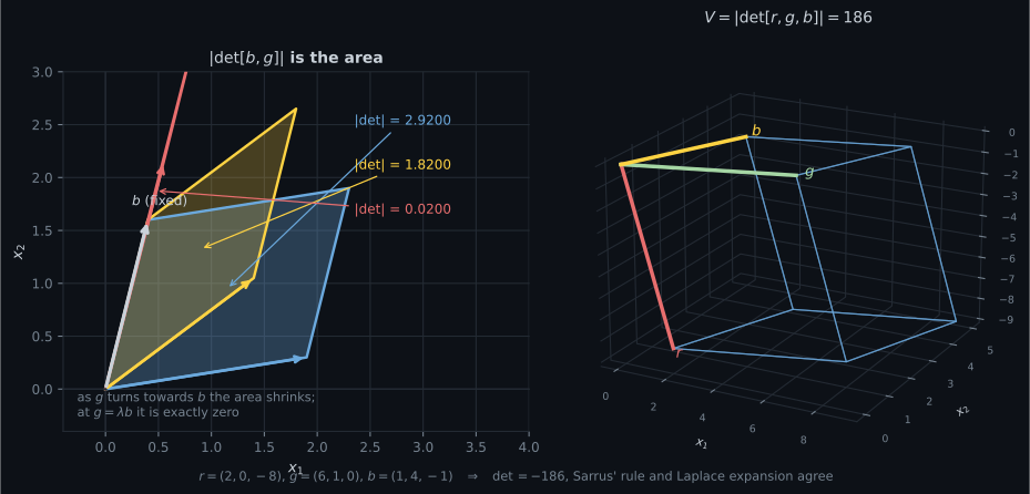
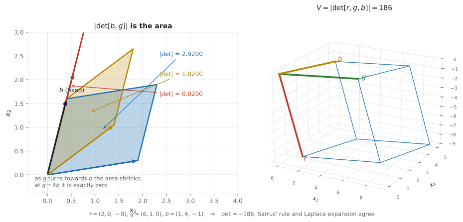
Reading the plot

From the volume figure. The left panel is the collapse. One vector is held fixed and the other is swung towards it: the areas measure $2.92$, $1.82$, $0.02$. At exact parallelism the determinant is $0.0$ to machine zero, and the matrix is singular — not “nearly singular”, singular, because the two columns are then linearly dependent and the rank drops.

The right panel is Example 4.2 verified, and it is worth reading the sign. The determinant is $-186$, not $+186$; the book quotes $V = \lvert\det\mathbf{A}\rvert = 186$ because volume is unsigned. The negative sign says $(\mathbf{r},\mathbf{g},\mathbf{b})$ is a left-handed frame — swap any two of them and it becomes right-handed with determinant $+186$.

From the cost figure. Read the ratio column of the table above, not the curves. The crossover is at $n = 4$: below that the Laplace recursion is genuinely competitive, which is why hand calculation uses it and why it does not feel like a bad idea. The reference lines confirm the asymptotics — the Laplace curve sits just above $n!$ and the elimination curve just above $n^3/3$.

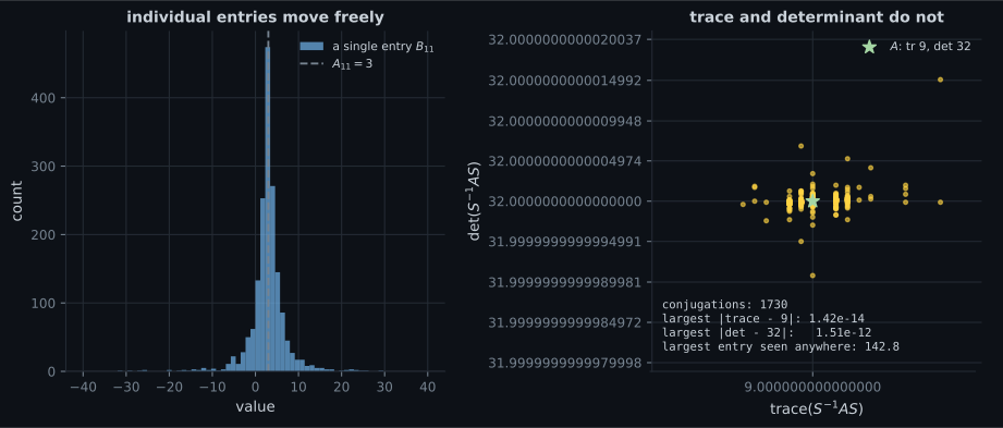
From the basis-change figure. This is the one to take seriously. The left histogram shows a single entry of $\mathbf{S}^{-1}\mathbf{A}\mathbf{S}$ ranging from $-31.9$ to $+62.0$, against an original value of $3$; somewhere in the sample an entry reached $142.9$. The matrix is being scrambled beyond recognition.

The right panel is the same $1730$ matrices plotted by trace and determinant, zoomed until floating-point noise is visible. Every point is on top of the original: the trace moved by at most $1.4\times10^{-14}$ and the determinant by at most $1.5\times10^{-12}$.

So “invariant under a change of basis” is not a mild statement. Under conjugation the matrix retains almost nothing recognisable, and these two numbers retain everything. That is why the chapter opens with them, and it is the same argument that will promote the eigenvalues in §4.2.

Pitfalls

Do not compute determinants to test invertibility

abs(det(A)) < tol is a bad singularity test. The determinant scales like $\lambda^n$, so a well-conditioned $50\times50$ matrix with entries around $10$ has a determinant around $10^{50}$ and a perfectly singular one scaled down by $10^{-2}$ has a determinant around $10^{-50}$ — the magnitude tells you about scale, not conditioning. Use np.linalg.cond, or a rank computed from an SVD. The Solving Systems page measures what conditioning actually costs.

The determinant overflows long before the matrix is large

For a $150\times150$ symmetric positive definite matrix, np.linalg.det returns inf while the matrix is perfectly well behaved. The fix is to work with $\log\det$ — for an SPD matrix, $2\sum_i \log L_{ii}$ from a Cholesky factor, which the Cholesky page measures out to $n = 175$ without trouble. Every Gaussian log-likelihood in Chapter 6 is written this way for exactly this reason.

The bars in the determinant notation are not an absolute value

The book puts this in a margin note because it catches people. $\lvert\mathbf{A}\rvert$ is the determinant, which is routinely negative. $\lvert\det\mathbf{A}\rvert$ is the volume.

The trace of a product is not the product of the traces

$\mathrm{tr}(\mathbf{A}\mathbf{B}) \neq \mathrm{tr}(\mathbf{A})\mathrm{tr}(\mathbf{B})$ in general — the determinant is multiplicative and the trace is additive, and mixing the two up is common. What the trace has instead is cyclic invariance, $\mathrm{tr}(\mathbf{A}\mathbf{K}\mathbf{L}) = \mathrm{tr}(\mathbf{K}\mathbf{L}\mathbf{A})$, which is a different and often more useful property.

Cyclic invariance is cyclic, not arbitrary

$\mathrm{tr}(\mathbf{A}\mathbf{B}\mathbf{C}) = \mathrm{tr}(\mathbf{B}\mathbf{C}\mathbf{A}) = \mathrm{tr}(\mathbf{C}\mathbf{A}\mathbf{B})$, and not $\mathrm{tr}(\mathbf{A}\mathbf{C}\mathbf{B})$. Rotating the sequence is allowed; reordering it is not. This bites when simplifying gradient expressions in Chapter 5.

Reach for Equation 4.20 before allocating an outer product

$\mathrm{tr}(\mathbf{x}\mathbf{y}^\top) = \mathbf{y}^\top\mathbf{x}$. The left-hand side builds an $n\times n$ matrix and reads $n$ of its $n^2$ entries; the right-hand side builds nothing. For $n = 400$ that is $160{,}000$ numbers against none, and the same substitution generalises — any trace of a product of thin matrices can usually be reordered into something small.

Compare

	determinant	trace
definition	signed volume, Equation 4.1	sum of the diagonal, Equation 4.18
defined for	square matrices only	square matrices only
on a sum	no simple rule	additive: $\mathrm{tr}(\mathbf{A}+\mathbf{B}) = \mathrm{tr}\mathbf{A} + \mathrm{tr}\mathbf{B}$
on a product	multiplicative: $\det\mathbf{A}\det\mathbf{B}$	cyclic: $\mathrm{tr}(\mathbf{A}\mathbf{B}) = \mathrm{tr}(\mathbf{B}\mathbf{A})$
on a scalar multiple	$\lambda^n \det\mathbf{A}$	$\lambda\,\mathrm{tr}\mathbf{A}$
basis independent?	yes	yes
in terms of eigenvalues	$\prod_i \lambda_i$ (Thm 4.16)	$\sum_i \lambda_i$ (Thm 4.17)
cost	$O(n^3)$ by elimination	$O(n)$
tests invertibility?	yes, in principle	no
overflows?	routinely, past $n \approx 150$	no

pch.quizTag Check your understanding

1. The book derives the 2x2 determinant from the formula for the inverse. Why is that the right way round?

   A It is not; the determinant is defined first B Because the determinant is precisely the quantity that has to be nonzero for the inverse to exist — Equation 4.2 has it as a denominator, and Equation 4.3 names the condition C Because 2x2 matrices are always invertible D Because the inverse is easier to compute
   pch.quizShowAnswer

   B — Because the determinant is precisely the quantity that has to be nonzero for the inverse to exist — Equation 4.2 has it as a denominator, and Equation 4.3 names the condition — Theorem 4.1 then generalises it: A is invertible if and only if det A is nonzero, and Theorem 4.3 adds that this is the same as having full rank.

2. Which three determinant properties license Gaussian elimination as a determinant algorithm?

   A Multiplicativity, transposition invariance, and the inverse rule B Adding a multiple of a row to another leaves it unchanged, scaling a row scales it, and swapping two rows flips its sign — so you can reach triangular form while tracking exactly what happened C Only the triangular product formula D The Laplace expansion
   pch.quizShowAnswer

   B — Adding a multiple of a row to another leaves it unchanged, scaling a row scales it, and swapping two rows flips its sign — so you can reach triangular form while tracking exactly what happened — Measured on random 5x5 matrices: row addition changed the determinant by 3.6e-15, a row swap gave a ratio of exactly -1, and scaling a row by 4 gave exactly 4.

3. tr(AB) = tr(BA) for A of shape 4x6 and B of shape 6x4. What is odd about that statement?

   A Nothing; both products are 4x4 B AB is 4x4 and BA is 6x6 — two matrices of different sizes with the same trace, measured here as -1.5121771480 for both C It only holds for square A and B D It requires A and B to commute
   pch.quizShowAnswer

   B — AB is 4x4 and BA is 6x6 — two matrices of different sizes with the same trace, measured here as -1.5121771480 for both — It generalises to invariance under cyclic permutation, and specialises for vectors to tr(x y-transpose) = y-transpose x — the identity that lets you avoid building an outer product at all.

4. Under two thousand random changes of basis, one entry of the matrix ranged over -31.9 to 62.0 while the trace moved by at most 1.4e-14. What is the significance?

   A The conjugations were badly conditioned B The matrix retains almost nothing recognisable under conjugation, and the trace and determinant retain everything — so they are properties of the linear mapping rather than of its representation C The trace is easier to compute than an entry D Nothing; all matrices behave this way
   pch.quizShowAnswer

   B — The matrix retains almost nothing recognisable under conjugation, and the trace and determinant retain everything — so they are properties of the linear mapping rather than of its representation — Equation 4.21 proves it in one line from cyclic invariance. It is also the argument that promotes the eigenvalues in section 4.2, which are invariant for the same reason.

🧪 Try It Yourself

Exercise 1 – Laplace expansion by hand

pch.exerciseTag pch.exerciseTitle

Exercise 2 – Verify the seven properties

pch.exerciseTag pch.exerciseTitle

Exercise 3 – Laplace against elimination

pch.exerciseTag pch.exerciseTitle

Exercise 4 – The trace identity worth memorising

pch.exerciseTag pch.exerciseTitle

Exercise 5 – Basis independence, measured

pch.exerciseTag pch.exerciseTitle

Recall card

• The determinant is a signed volume: the absolute value is the volume of the parallelepiped spanned by the columns, and the sign records orientation.
• det A nonzero, invertible, and full rank are the same condition — Theorems 4.1 and 4.3.
• For a triangular matrix the determinant is the product of the diagonal, which is why Gaussian elimination is the practical algorithm.
• The Laplace expansion is correct and costs about n factorial. At n = 20 that is 4.2e18 multiplications against 2679 for elimination — the book says numerical methods superseded the explicit determinant, and this is the size of the reason.
• Three row operations have known effects: adding a multiple of a row changes nothing, scaling a row scales the determinant, swapping two rows flips its sign.
• The trace is the sum of the diagonal, is additive rather than multiplicative, and is the only function satisfying its four listed properties.
• The trace is invariant under cyclic permutation, so tr(AB) equals tr(BA) even when the two products have different sizes; for vectors it collapses to tr(x y-transpose) = y-transpose x.
• Both the determinant and the trace survive a change of basis — measured, a single entry roamed over a range of 94 while the trace held to fourteen decimals.
• They are two coefficients of the characteristic polynomial: the constant term is the determinant and the next-to-leading one is plus or minus the trace.

Next: Eigenvalues and Eigenvectors — the roots of that polynomial, and what they mean.