Key Steps of PCA in Practice

Six pages of derivation collapse into one recipe. §10.6 lists it, and two of its steps are not bookkeeping:

Step 2 changes the answer. The book calls it “standardization” and moves on. Measured below, skipping it lets a change of units rotate the leading direction by $77.3982^\circ$ on data that never moved.

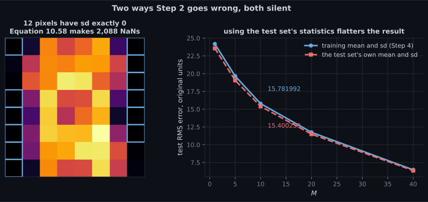
Step 4 says whose mean and standard deviation to use. “We need to standardize $\mathbf{x}_*$ using the mean $\mu_d$ and standard deviation $\sigma_d$ of the training data.” Using the test set’s own statistics instead makes the reported error smaller, which is why the mistake survives.

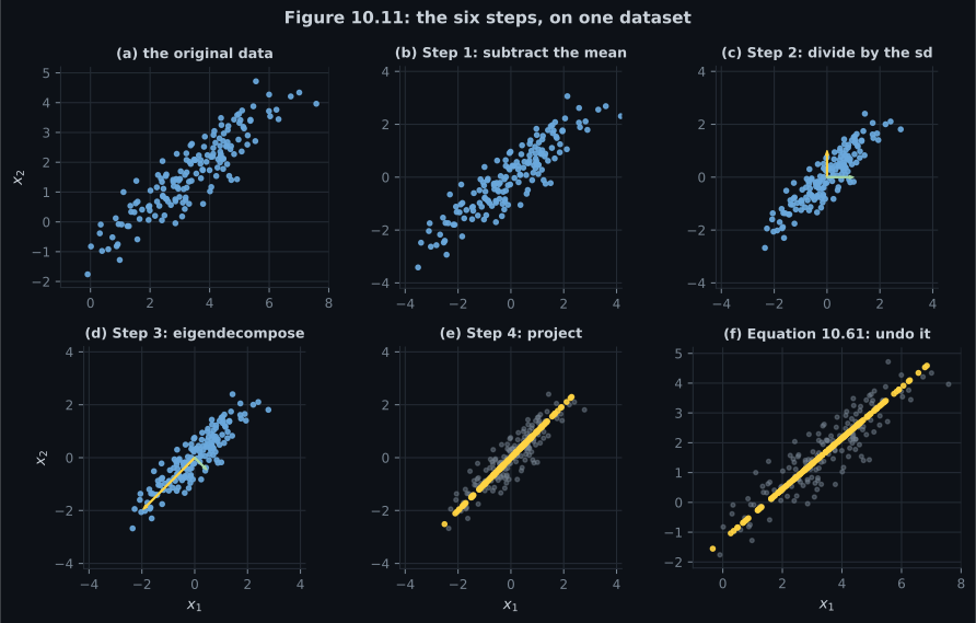
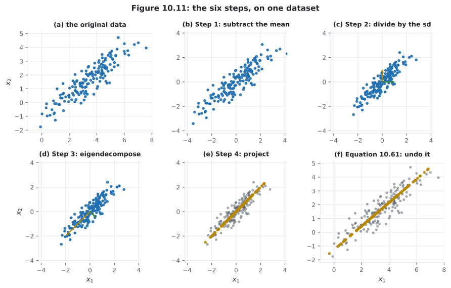
What you’ll learn

• The six steps as Figure 10.11 draws them, run end to end on one dataset.
• Why Step 1’s “not strictly necessary but reduces the risk of numerical problems” understates it — page 1001 already measured the $87.9996^\circ$ swing.
• What Step 2 actually does: standardising then computing the covariance gives the correlation matrix, measured to $6.7\times10^{-16}$, and pins the total variance at exactly $D$.
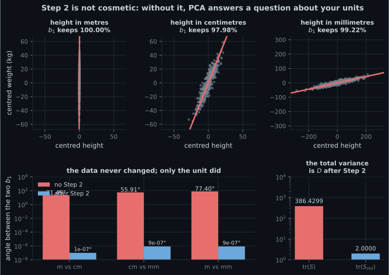
• Measured on height and weight: unstandardised, the leading direction is $[0.003887, 0.999992]$ in metres and $[0.976750, 0.214380]$ in millimetres — $77.3982^\circ$ apart. Standardised, all three unit choices agree to $1.2\times10^{-6}$ degrees.
• Equations 10.58–10.61, the forward and inverse maps, with a round trip measured at $2.3\times10^{-14}$ when $M = D$.
• Two silent failures: dividing by a zero standard deviation produces $2{,}088$ NaNs on the digit-”8” images, and using the test set’s own statistics reports $15.400250$ where the honest figure is $15.781992$.
• The sentence at the end of Step 4: “PCA returns the coordinates (10.60), not the projections.”

Intuition: PCA has no idea what your columns mean

Everything from §10.2 onward maximises variance, and variance has units. A column measured in millimetres has a variance a million times larger than the same column in metres — so an unstandardised PCA will point at whichever column happens to be recorded in the smallest unit.

Standardising sets every column’s variance to $1$, which makes the question “which direction varies most” meaningful across columns that measure different things. It is a decision, not a correction: you are declaring that a one-standard-deviation move is equally important in every variable.

diagram The six steps, and where each one can go wrong mermaid

  flowchart TD
  A["1. subtract the mean
page 1001: 87.9996 degrees if you skip it"]
  A --> B["2. divide by the sd
77.3982 degrees if you skip it
NaN if any sd is 0"]
  B --> C["3. eigendecompose S
page 1005: SVD, not eigh, if kappa is large"]
  C --> D["4. project: z = B'x
with the TRAINING mu and sigma"]
  D --> E["Eq 10.61: undo the standardisation
only if you want pictures"]
  D --> F["PCA returns z, not x~"]

§10.6 The six steps

1. Mean subtraction. “This ensures that the dataset has mean $\mathbf{0}$. Mean subtraction is not strictly necessary but reduces the risk of numerical problems.”

2. Standardization. Divide by the standard deviation $\sigma_d$ in every dimension. “Now the data is unit free, and it has variance $1$ along each axis.”

3. Eigendecomposition of the covariance matrix. By the spectral theorem an ONB of eigenvectors exists; §10.4 covered how to obtain it.

4. Projection. For any $\mathbf{x}_*$:

$$x_*^{(d)} \leftarrow \frac{x_*^{(d)} - \mu_d}{\sigma_d}, \qquad d = 1,\ldots,D \qquad \text{(10.58)}$$ $$\tilde{\mathbf{x}}_* = \mathbf{B}\mathbf{B}^\top\mathbf{x}_*, \qquad \mathbf{z}_* = \mathbf{B}^\top\mathbf{x}_* \qquad \text{(10.59), (10.60)}$$

PCA returns the coordinates (10.60), not the projections $\mathbf{x}_*$.

5. Undoing the standardization, if you want the picture back in the original space:

$$\tilde{x}_*^{(d)} \leftarrow \tilde{x}_*^{(d)}\sigma_d + \mu_d, \qquad d = 1,\ldots,D \qquad \text{(10.61)}$$

figure Figure 10.11, run end to end matplotlib

Panels (c) and (d) hold the same points and differ only in what is drawn on them: the unit-variance axes Step 2 creates, then the eigenvectors Step 3 finds, scaled by the square roots of their eigenvalues. Panel (f) is Equation 10.61 — the projection carried back through the standardisation, which is why the orange line in (f) is not at 45 degrees.

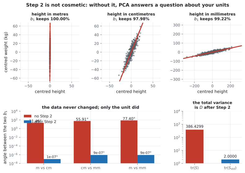
Step 2 is a modelling decision

Take two genuinely different quantities — height and weight — with a correlation of $0.9198$, and vary nothing but the unit of the first column:

units of height	leading direction $\mathbf{b}_1$	share of variance it keeps
metres	$[0.003887,\ 0.999992]$	$100.00\%$
centimetres	$[0.369903,\ 0.929070]$	$97.98\%$
millimetres	$[0.976750,\ 0.214380]$	$99.22\%$

angle between two unstandardised answers	degrees
metres vs centimetres	$21.49$
centimetres vs millimetres	$55.91$
metres vs millimetres	$\mathbf{77.3982}$

Standardise first, and all three become $[0.707107,\ 0.707107]$ keeping $95.99\%$ — agreeing to $1.2\times10^{-6}$ degrees.

figure The same data, three units, three different first principal components matplotlib

Nothing about the data changed between the top three panels — only the number written on the height axis. Unstandardised PCA reports whichever column happens to carry the largest numbers. After Step 2 the three answers are the same direction to a millionth of a degree, and the total variance is exactly D.

What Step 2 is really doing

Standardising and then forming Equation 10.1 gives the correlation matrix, not the covariance — measured agreement with np.corrcoef, $6.7\times10^{-16}$:

	raw covariance	after Step 2
the matrix	$\begin{bmatrix}0.0069 & 1.5019\\ 1.5019 & 386.4230\end{bmatrix}$	$\begin{bmatrix}1 & 0.9198\\ 0.9198 & 1\end{bmatrix}$
its trace	$386.429897$, in $\mathrm{m}^2 + \mathrm{kg}^2$	$2.000000$, i.e. exactly $D$

That first trace is the giveaway. It has no units — it is a sum of a squared length and a squared mass — so “the fraction of variance explained” computed from it is a ratio of two quantities that mean nothing. After Step 2 the trace is $D$ for any dataset, and the fraction is a genuine share.

The trade-off is real and worth stating: standardising discards the information that one variable really does vary more than another. When the columns share a unit — pixel intensities, say, or prices — that information is meaningful and §10.6’s Step 2 is the wrong default. The digit pages in this chapter do not standardise, for exactly that reason.

Two silent failures

A zero standard deviation

Equation 10.58 divides by $\sigma_d$. On the digit-”8” images, page 1001 measured $12$ pixels with variance exactly zero:

	value
pixels with $\sigma_d = 0$	$12$ of $64$
NaNs produced by Equation 10.58	$\mathbf{2{,}088}$ ($= 12 \times 174$)
infinities produced	$0$

Every NaN is $0/0$, not a division of a nonzero number. np.linalg.eigh on the result raises nothing useful; replacing the NaNs with zeros runs and decomposes a matrix built from values you invented. The fix is to drop the constant dimensions first — they carry no information by construction, so removing them costs nothing.

figure Both of these fail without raising anything matplotlib

Left: the outlined border pixels are black in every image, so Equation 10.58 divides zero by zero for each of them. Right: standardising the test set with its own mean and standard deviation reports a lower error at every M — 15.400250 against 15.781992 at M = 10 — because it has quietly re-centred the test set in a frame the basis was never fitted in.

The wrong mean and standard deviation

Step 4 is explicit that $\mu_d$ and $\sigma_d$ come from the training data. Measured on a $140/34$ split of the digit-”8” images at $M = 10$:

standardising the test set with	test RMS error, original units
the training mean and sd — Step 4 as written	$15.781992$
the test set’s own mean and sd	$\mathbf{15.400250}$

The wrong answer is the better-looking one

The difference is $-0.381741$: the leak makes the model look better, which is why it survives code review. The test set’s mean differs from the training mean by $5.900273$ and its per-pixel standard deviations by up to $1.207279$, so re-standardising moves it into a frame that fits its own spread slightly better than the frame $\mathbf{B}$ was fitted in.

The resulting number is not wrong by $0.38$ — it is not a measurement of anything, because the basis and the data are now in different coordinate systems. And the effect grows with how much the two sets differ, so a small test set makes it worse precisely when you can least afford it.

The round trip

Equations 10.58 → 10.60 → 10.59 → 10.61, on the same split, reporting the error back in the original pixel units:

$M$	test RMS reconstruction error
$1$	$24.179252$
$5$	$19.658189$
$10$	$15.781992$
$20$	$11.748255$
$40$	$6.473157$
$64$	$\mathbf{3.3\times10^{-14}}$

The last row is the check that matters: with every component kept, the whole pipeline — centre, standardise, project, unproject, unstandardise — is the identity to floating point. (The exact figure drifts in the last couple of digits between runs; what matters is that it is at machine level and not, say, $10^{-6}$.)

Which number does PCA actually hand you?

PCA returns the coordinates (10.60), not the projections $\mathbf{x}_*$.

$\mathbf{z}_* = \mathbf{B}^\top\mathbf{x}_*$ is $M$ numbers; $\tilde{\mathbf{x}}_* = \mathbf{B}\mathbf{z}_*$ is $D$ numbers with only $M$ degrees of freedom, which page 1001 measured as a rank-$M$ matrix.

For one test image at $M = 10$, the code is

$$[3.8604,\ -2.1537,\ 4.4452,\ -0.8718,\ 2.6041,\ -2.2010,\ 0.2211,\ 2.9317,\ 1.1960,\ -0.0958]$$

That is what goes into the next model, the plot, or the index. The reconstruction exists only so you can look at it — Equation 10.61’s whole job is producing Figure 10.11(f) and Figure 10.12.

pch.quizTag Is the recipe clear?

1. Why does Step 2 matter beyond being tidy?

   A It speeds up the eigendecomposition B Without it the answer depends on the units — measured, a metres-to-millimetres change rotates the leading direction 77.3982 degrees C It is required for the eigenvectors to be orthogonal D It removes outliers
   pch.quizShowAnswer

   B — Without it the answer depends on the units — measured, a metres-to-millimetres change rotates the leading direction 77.3982 degrees — Variance has units, so a column recorded in a smaller unit has a larger variance and attracts the leading direction. In metres it comes out as [0.003887, 0.999992] and in millimetres as [0.976750, 0.214380] — the same data both times. After Step 2 the three unit choices agree to 1.2e-06 degrees.

2. What matrix does the standardised data's covariance equal?

   A The identity B The correlation matrix, and its trace is exactly D for any dataset C The inverse covariance D The Gram matrix
   pch.quizShowAnswer

   B — The correlation matrix, and its trace is exactly D for any dataset — Measured to 6.7e-16. That is why the fraction-of-variance figure only means something after Step 2: the raw trace on height and weight was 386.429897 in units of squared metres plus squared kilograms, which is not a quantity. The cost is that you have declared a one-standard-deviation move equally important in every column.

3. What happens if a dimension has zero variance and you apply Equation 10.58?

   A Nothing; the column becomes zero B You divide zero by zero — 2,088 NaNs on the digit-8 images, with no error raised C You get infinities D numpy raises a ZeroDivisionError
   pch.quizShowAnswer

   B — You divide zero by zero — 2,088 NaNs on the digit-8 images, with no error raised — Twelve of the sixty-four pixels are black in every image, giving 12 times 174 NaNs. No exception is raised; replacing them with zeros produces a decomposition of numbers you invented. Drop the constant dimensions first — they carry no information by construction.

4. Step 4 says to standardise a new point with the training mean and standard deviation. What goes wrong otherwise?

   A The error goes up sharply B The reported error goes DOWN — 15.400250 against an honest 15.781992 — and stops measuring anything C The code has the wrong length D The eigenvectors change
   pch.quizShowAnswer

   B — The reported error goes DOWN — 15.400250 against an honest 15.781992 — and stops measuring anything — That is what makes the mistake durable: it flatters the result. The basis was fitted in the training coordinate frame, and re-standardising the test set moves it into a different frame that fits its own spread slightly better. The training and test means here differ by 5.900273.

Exercises

Exercise 1 – Change the unit, change the answer

pch.exerciseTag pch.exerciseTitle

Exercise 2 – What Step 2 turns the covariance into

pch.exerciseTag pch.exerciseTitle

Exercise 3 – Dividing by zero, quietly

pch.exerciseTag pch.exerciseTitle

Exercise 4 – The round trip, in the original units

pch.exerciseTag pch.exerciseTitle

Exercise 5 – Whose mean and standard deviation

pch.exerciseTag pch.exerciseTitle

Recall card

• Section 10.6 is the recipe: centre, standardise, eigendecompose, project with the training statistics, and optionally undo the standardisation to get a picture back.
• Step 2 is a modelling decision, not tidiness. Variance carries the square of whatever unit you wrote down, so an unstandardised PCA points at whichever column has the largest numbers.
• Measured, switching height from metres to millimetres rotates the leading direction 77.3982 degrees on data that never moved. After standardising, three unit choices agree to about a millionth of a degree.
• Standardising and then computing Equation 10.1 gives the correlation matrix, matched to 6.7e-16, and its trace is exactly D for every dataset.
• Which is why a percentage of variance explained only means something after Step 2 — the raw trace on height and weight was a sum of squared metres and squared kilograms.
• But the trade-off is real: when the columns share a unit, the fact that one varies more is information, and standardising throws it away. The digit pages in this chapter do not standardise.
• A zero standard deviation makes Equation 10.58 compute zero over zero. On the digit-8 images that is 2,088 NaNs and no exception. Drop the constant columns first.
• Step 4 says to use the training mean and standard deviation for any new point, and the failure mode is the dangerous kind: using the test set’s own statistics reports 15.400250 where the honest number is 15.781992.
• A leak that flatters the result is the one that survives code review.
• Kept in full, the pipeline is the identity to about 3e-14 — the check worth writing whenever you implement it.
• PCA returns the coordinates, not the projections. The code is M numbers; the reconstruction is D numbers with only M degrees of freedom, and exists so you can look at it.

Next: The Latent Variable Perspective — §10.7 puts a probabilistic model behind all of this, and recovers everything so far as the noise-free limit.