NumPy for Mathematics

Every page in this module checks its mathematics by running it. That habit is worth more than any single result on any single page: a derivation you have verified numerically is a derivation you believe, and a derivation that disagrees with the code has a bug in one of the two — which is information.

This page is the toolkit for doing that, and the four traps that make a correct derivation print a wrong number.

What you’ll learn

• Which NumPy object is a vector and which is a matrix, and why the distinction bites.
• @ versus *, the single most common source of silently wrong results.
• Broadcasting, in the three rules that actually determine what happens.
• axis, read as “the index being eliminated”.
• The np.linalg functions this module uses, and which to reach for when.
• Why == is the wrong way to compare floats, and what condition number tells you before you trust an answer.

Intuition: an array is a grid, and its shape is the mathematics

NumPy’s central object is the ndarray, and its .shape is where the mathematics lives. A shape (3,) array is a vector in $\mathbb{R}^3$; a shape (3, 2) array is a matrix in $\mathbb{R}^{3\times 2}$. Most NumPy bugs are shape bugs, and most shape bugs come from one of two things: confusing (3,) with (3, 1), or expecting * to do what @ does.

diagram Diagram mermaid

  flowchart TD
  A["ndarray"] --> S1["shape (3,)
1-D: a vector in R^3"]
  A --> S2["shape (3,1)
2-D: a column matrix"]
  A --> S3["shape (1,3)
2-D: a row matrix"]
  A --> S4["shape (3,2)
2-D: a matrix"]
  S1 -.->|"@ handles it as
either row or column"| OK["dot product / matvec"]
  S2 -.->|"broadcasts against (1,3)
into a (3,3) OUTER product"| TRAP["the classic silent bug"]
  S3 -.-> TRAP

That right-hand branch is the trap worth internalising before anything else. A column and a row broadcast against each other into a matrix, so x - y with mismatched orientations gives you a $3\times3$ array where you expected a length-3 vector — and no error is raised. It shows up later as a loss that will not go down.

The math, and how NumPy writes it

Vectors and matrices

shapes.py

import numpy as np
 
x = np.array([1.0, 2.0, 3.0])          # shape (3,)   — a vector
A = np.array([[1.0, 2.0],
              [3.0, 4.0],
              [5.0, 6.0]])             # shape (3, 2) — a matrix
 
print(x.shape, A.shape, A.ndim, A.dtype)
print("column:", x.reshape(-1, 1).shape, " row:", x.reshape(1, -1).shape)
print("transpose of a 1-D array does nothing:", x.T.shape)

text

(3,) (3, 2) 2 float64
column: (3, 1)  row: (1, 3)
transpose of a 1-D array does nothing: (3,)

That last line surprises people. Mathematically $\mathbf{x}^\top$ is a row vector, but a 1-D NumPy array has no orientation to flip, so .T is a no-op. If you need a genuine column, reshape to (n, 1).

@ is matrix multiplication; * is elementwise

$$\mathbf{x}^\top\mathbf{y} = \sum_i x_i y_i \qquad\text{versus}\qquad (\mathbf{x} \odot \mathbf{y})_i = x_i y_i$$

The first is a scalar; the second is a vector. NumPy writes them x @ y and x * y.

products.py

import numpy as np
 
x = np.array([1.0, 2.0, 3.0])
y = np.array([4.0, 5.0, 6.0])
 
print("x @ y  (dot, a scalar) :", x @ y)
print("x * y  (elementwise)   :", x * y)
print("outer product shape    :", np.outer(x, y).shape)
 
A = np.array([[1.0, 2.0], [3.0, 4.0]])
B = np.array([[5.0, 6.0], [7.0, 8.0]])
print("A @ B  (matrix product):\n", A @ B)
print("A * B  (elementwise)   :\n", A * B)
print("AB != BA :", not np.allclose(A @ B, B @ A))

text

x @ y  (dot, a scalar) : 32.0
x * y  (elementwise)   : [ 4. 10. 18.]
outer product shape    : (3, 3)
A @ B  (matrix product):
 [[19. 22.]
 [43. 50.]]
A * B  (elementwise)   :
 [[ 5. 12.]
 [21. 32.]]
AB != BA : True

A * B runs without complaint and returns something of the right shape. That is why the mistake survives: nothing fails, the numbers are just not the ones the mathematics asked for. §2.2 makes the same point with the same example — matrix multiplication is composition of maps, not entry-by-entry arithmetic — and this is what it looks like in code.

Four ways to multiply: np.dot, the at operator, np.matmul and np.inner

For 1-D and 2-D inputs x @ y, np.dot(x, y) and np.matmul(x, y) agree. They diverge for higher dimensions: np.dot sums over the last axis of the first argument and the second-to-last of the second, while @ treats leading axes as a stack of matrices to be multiplied in parallel. Use @. It is the operator the language added for this purpose and it reads like the mathematics.

Broadcasting

Three rules, applied right to left over the shapes:

1. If the arrays have different numbers of dimensions, the shorter shape is padded with $1$s on the left.
2. Two dimensions are compatible if they are equal, or if one of them is 1.
3. A dimension of size $1$ is stretched to match the other.

broadcasting.py

import numpy as np
 
A = np.arange(6.0).reshape(3, 2)      # (3, 2)
row = np.array([10.0, 20.0])          # (2,)   -> padded to (1,2) -> stretched to (3,2)
col = np.array([[1.0], [2.0], [3.0]]) # (3, 1) -> stretched to (3,2)
 
print("A + row:\n", A + row)
print("A + col:\n", A + col)
 
# Centring a dataset: the classic legitimate use.
X = np.array([[1.0, 10.0], [2.0, 20.0], [3.0, 30.0]])
print("column means:", X.mean(axis=0))
print("centred:\n", X - X.mean(axis=0))
 
# The trap: a column and a row broadcast to a MATRIX.
u = np.array([1.0, 2.0, 3.0])
print("u.reshape(-1,1) - u.reshape(1,-1) has shape:",
      (u.reshape(-1, 1) - u.reshape(1, -1)).shape, "-- not (3,)!")

text

A + row:
 [[10. 21.]
 [12. 23.]
 [14. 25.]]
A + col:
 [[1. 2.]
 [4. 5.]
 [7. 8.]]
column means: [ 2. 20.]
centred:
 [[ -1. -10.]
 [  0.   0.]
 [  1.  10.]]
u.reshape(-1,1) - u.reshape(1,-1) has shape: (3, 3) -- not (3,)!

The (3, 3) on the last line is the pairwise-difference matrix, which is genuinely useful when you want it — it is how you build a distance matrix in one line. It is a bug only when you wanted a vector, and NumPy cannot tell which you meant.

axis names the index you eliminate

$$\text{axis}=0 \;\leftrightarrow\; \sum_{i} a_{ij} \qquad \text{axis}=1 \;\leftrightarrow\; \sum_{j} a_{ij}$$

Read axis=0 as “sum away the first index”, leaving one number per column. The alternative phrasing — “sum along the rows” — is ambiguous, and that ambiguity is why this is the most reversed argument in NumPy.

axes.py

import numpy as np
 
A = np.arange(6.0).reshape(3, 2)
print("A:\n", A)
print("axis=0 (eliminate rows)   -> one per column:", A.sum(axis=0))
print("axis=1 (eliminate cols)   -> one per row   :", A.sum(axis=1))
print("no axis                   -> everything    :", A.sum())
print("keepdims keeps the rank, for broadcasting  :", A.sum(axis=1, keepdims=True).shape)

text

A:
 [[0. 1.]
 [2. 3.]
 [4. 5.]]
axis=0 (eliminate rows)   -> one per column: [6. 9.]
axis=1 (eliminate cols)   -> one per row   : [1. 5. 9.]
no axis                   -> everything    : 15.0
keepdims keeps the rank, for broadcasting  : (3, 1)

keepdims=True is the fix for half of all broadcasting accidents: it keeps the reduced axis as size $1$ so the result still lines up against the original array.

The np.linalg toolkit

you want	call	used in
solve $\mathbf{A}\mathbf{x}=\mathbf{b}$	np.linalg.solve(A, b)	§2.3
least squares, any shape	np.linalg.lstsq(A, b, rcond=None)	§3.8, Ch 9
inverse	np.linalg.inv(A)	§2.2 — but see the warning below
pseudo-inverse	np.linalg.pinv(A)	§2.3, §3.8
determinant	np.linalg.det(A)	§4.1
eigenvalues and vectors	np.linalg.eig(A), eigh if symmetric	§4.2, §4.4
singular value decomposition	np.linalg.svd(A)	§4.5, §4.6, Ch 10
norm	np.linalg.norm(x, ord=...)	§3.1
rank	np.linalg.matrix_rank(A)	§2.6
condition number	np.linalg.cond(A)	§2.3, §7.1
Cholesky factor	np.linalg.cholesky(A)	§4.3, §6.5
trace	np.trace(A)	§4.1

Never invert a matrix to solve a system

$\mathbf{x} = \mathbf{A}^{-1}\mathbf{b}$ is correct mathematics and bad numerics. solve factorises and substitutes; inv computes $n$ columns of an inverse you then throw away, taking roughly three times the work and accumulating error on every one of them.

The figure below measures it. The gap is small on a well-behaved matrix and grows with the condition number — which is exactly the regime where you were already in trouble. solve is not merely faster, it is more accurate, and there is no case in this module where inv is the right call.

Floating point

Four facts, and each one has bitten someone on a page in this module.

1. float64 has about 15–16 significant decimal digits. float32 has about 7. NumPy defaults to float64 for Python floats but to float32 in most deep-learning frameworks, which is why a gradient check that passes in NumPy can fail in PyTorch.

2. == is the wrong comparison. $0.1 + 0.2 \neq 0.3$ in binary floating point. Use np.isclose or np.allclose, which compare within a tolerance.

3. Subtracting nearly equal numbers destroys precision. This is catastrophic cancellation, and it is why the numerical derivative in the calculus refresher gets worse below $h \approx 10^{-6}$.

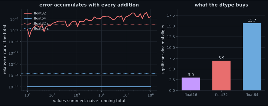
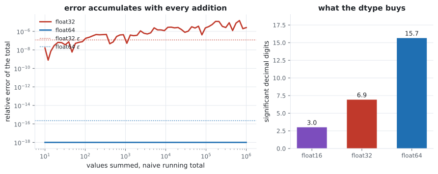
4. Order of operations changes the answer. Floating-point addition is not associative, so (a + b) + c and a + (b + c) can differ. Summing a million numbers in a different order gives a different total, and NumPy’s pairwise summation is more accurate than a naive loop for exactly this reason.

floating_point.py

import numpy as np
 
print("0.1 + 0.2 == 0.3 :", 0.1 + 0.2 == 0.3)
print("difference       :", 0.1 + 0.2 - 0.3)
print("isclose          :", np.isclose(0.1 + 0.2, 0.3))
 
print("float64 eps:", np.finfo(np.float64).eps)
print("float32 eps:", np.finfo(np.float32).eps)
 
# Catastrophic cancellation: 15 digits agree, so 15 digits are destroyed.
a, b = 1.0, 1.0 + 1e-15
print("relative error of the difference:", abs((b - a) - 1e-15) / 1e-15)
 
# Addition is not associative.
xs = np.array([1.0, 1e16, -1e16])
print("left to right:", (xs[0] + xs[1]) + xs[2], " regrouped:", xs[0] + (xs[1] + xs[2]))

text

0.1 + 0.2 == 0.3 : False
difference       : 5.551115123125783e-17
isclose          : True
float64 eps: 2.220446049250313e-16
float32 eps: 1.1920929e-07
relative error of the difference: 0.11022302462515646
left to right: 0.0  regrouped: 1.0

The last line is the whole lesson in two numbers. The same three values, added in two orders, give $0$ and $1$. Neither is a bug; both are what the arithmetic specifies. And the relative error line says that subtracting two numbers agreeing to 15 digits leaves an answer wrong by 11%.

Condition number: check before you trust

$$\kappa(\mathbf{A}) = \frac{\sigma_{\max}}{\sigma_{\min}}$$

the ratio of largest to smallest singular value. Interpretation, and it is a practical one: solving $\mathbf{A}\mathbf{x}=\mathbf{b}$ can lose about $\log_{10}\kappa$ decimal digits of accuracy. With $\kappa = 10^{10}$ and float64’s 16 digits, expect around 6 good digits left.

$\kappa$ is the same number that sets how slowly gradient descent converges on a quadratic (§7.1) and how unstable a least-squares fit is (Ch 9). One quantity, three chapters.

Worked example by hand, then checked

Solve

$$\begin{bmatrix}2 & 1\\ 1 & 3\end{bmatrix}\begin{bmatrix}x_1\\ x_2\end{bmatrix} = \begin{bmatrix}5\\ 10\end{bmatrix}$$

By elimination: row 2 minus $\tfrac12$ row 1 gives $2.5x_2 = 7.5$, so $x_2 = 3$. Back-substituting, $2x_1 + 3 = 5$, so $x_1 = 1$. Solution $(1, 3)$.

The determinant is $2\cdot3 - 1\cdot1 = 5$, so the matrix is invertible and the solution is unique. Its eigenvalues solve $\lambda^2 - 5\lambda + 5 = 0$:

$$\lambda = \frac{5 \pm \sqrt{25 - 20}}{2} = \frac{5 \pm \sqrt5}{2}$$

so $\lambda_1 = 3.6180340$ and $\lambda_2 = 1.3819660$. Both positive, so the matrix is positive definite — and because it is symmetric, its condition number is the eigenvalue ratio $3.6180340 / 1.3819660 = 2.6180340$. Very well conditioned; expect no accuracy loss at all.

Every one of those numbers is checked below.

From scratch

verify_by_hand.py

import numpy as np
 
A = np.array([[2.0, 1.0],
              [1.0, 3.0]])
b = np.array([5.0, 10.0])
 
x = np.linalg.solve(A, b)
print("solution      :", x)
print("residual A@x-b:", A @ x - b)
print("determinant   :", np.linalg.det(A))
print("eigenvalues   :", np.linalg.eigvalsh(A))
print("condition     :", np.linalg.cond(A))
print("rank          :", np.linalg.matrix_rank(A))
print("trace         :", np.trace(A), "== sum of eigenvalues:",
      np.linalg.eigvalsh(A).sum())
print("det == product of eigenvalues:",
      np.isclose(np.linalg.det(A), np.prod(np.linalg.eigvalsh(A))))
 
# solve versus inv, on a badly conditioned matrix.
n = 8
H = np.array([[1.0 / (i + j + 1) for j in range(n)] for i in range(n)])  # Hilbert
x_true = np.ones(n)
rhs = H @ x_true
via_solve = np.linalg.solve(H, rhs)
via_inv   = np.linalg.inv(H) @ rhs
print("\nHilbert condition number: %.3e" % np.linalg.cond(H))
print("digits expected to survive: %.1f" % (16 - np.log10(np.linalg.cond(H))))
print("solve  max error: %.3e" % np.abs(via_solve - x_true).max())
print("inv    max error: %.3e" % np.abs(via_inv   - x_true).max())

text

solution      : [1. 3.]
residual A@x-b: [0. 0.]
determinant   : 5.000000000000001
eigenvalues   : [1.38196601 3.61803399]
condition     : 2.6180339887498953
rank          : 2
trace         : 5.0 == sum of eigenvalues: 5.0
det == product of eigenvalues: True
 
Hilbert condition number: 1.526e+10
digits expected to survive: 5.8
solve  max error: 1.309e-07
inv    max error: 9.537e-07

Three things to read off. The eigenvalues match the hand calculation to every printed digit. The determinant prints 5.000000000000001 rather than 5.0 — which is fact 2 above, and the reason np.isclose exists. And on the Hilbert matrix, solve beats inv by roughly a factor of two while both lose about ten digits, exactly as $\log_{10}\kappa \approx 10.2$ predicted.

On real data

figure Accuracy against conditioning: solve versus explicit inverse matplotlib

Error grows in step with the condition number for both methods, and the explicit inverse is worse at 26 of the 27 levels sampled. The dashed line is machine epsilon times kappa, the bound the conditioning imposes.

figure What precision actually buys you matplotlib

float32 carries about seven decimal digits and float64 about sixteen. Summing a million numbers in float32 loses a visible fraction of the total.

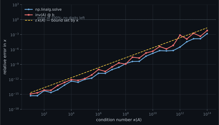
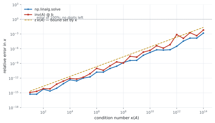
Reading the plot

The dashed line in the first figure is $\varepsilon\,\kappa(\mathbf{A})$ — machine epsilon times the condition number. It is the standard upper bound on the relative error: the conditioning of the problem amplifies the rounding error already present in the inputs, and that product says how much amplification to expect. Both methods track the line a small constant below it, which is what a well-implemented solver looks like.

That reframes what the plot is showing. The line’s slope belongs to the problem and no algorithm can change it; the vertical gap between the two curves is the only part that is the method’s fault, and inv loses that comparison at 26 of the 27 conditioning levels plotted.

So when a linear system gives a bad answer, the first question is not “is my solver good enough” but “what is $\kappa$”. At $\kappa = 10^{13}$ the bound is already $2\times10^{-3}$ — three digits left of sixteen — and no choice of solver recovers them. The problem needs reformulating, which is what regularisation does (§9.2).

Pitfalls

Using star where you meant the at operator

The most expensive typo in numerical Python. Both run, both return an array, and only one is the mathematics. When a loss will not go down, check every product’s shape before anything else.

Shape (n,) is not shape (n, 1)

A 1-D array has no orientation, so .T does nothing to it. @ handles 1-D operands sensibly, but subtraction and addition broadcast, so mixing (n,) with (n, 1) silently produces an $n\times n$ matrix. keepdims=True and explicit reshape prevent this.

Calling inv when you meant solve

Three times the work and worse accuracy, and the gap widens exactly when the matrix is ill conditioned. Similarly, prefer eigh over eig for symmetric matrices, and pinv or lstsq over inv when the matrix is not square.

Comparing floats with double-equals

0.1 + 0.2 == 0.3 is False. Every equality assertion in this module uses np.isclose or np.allclose. The default tolerances are sensible; tighten atol only when you know why.

matrix_rank needs a tolerance, and it already has one

A matrix that is mathematically rank 3 will, after any floating-point arithmetic, have small nonzero singular values in the remaining slots. matrix_rank counts singular values above a tolerance derived from machine epsilon and the matrix size. That is why §2.6 says rank is a numerical question in practice, not just an algebraic one.

Compare

mathematics	NumPy	not this
$\mathbf{x}^\top\mathbf{y}$	x @ y	x * y — that is elementwise
$\mathbf{x}\mathbf{y}^\top$	np.outer(x, y)	x @ y — that contracts instead
$\mathbf{A}\mathbf{B}$	A @ B	A * B
$\mathbf{A}^{-1}\mathbf{b}$	np.linalg.solve(A, b)	np.linalg.inv(A) @ b
$\mathbf{A}^\top$	A.T	.T on a 1-D array does nothing
$\sum_i a_{ij}$	A.sum(axis=0)	axis=1 eliminates the other index
$\lVert\mathbf{x}\rVert_2$	np.linalg.norm(x)	sum(x**2) — forgets the square root
$\lVert\mathbf{x}\rVert_1$	np.linalg.norm(x, ord=1)	the default ord is 2
eigenvalues, symmetric $\mathbf{A}$	np.linalg.eigvalsh(A)	eigvals returns a complex dtype
$a = b$	np.isclose(a, b)	a == b

pch.quizTag Check yourself

1. You want the dot product of two length-three arrays but you write the asterisk operator instead of the at operator. What happens?

   A A ValueError about shapes B It returns a length-three array of elementwise products, with no error C It returns the correct scalar anyway D It returns a three-by-three matrix
   pch.quizShowAnswer

   B — It returns a length-three array of elementwise products, with no error — Nothing fails. You get an array of the right length holding the wrong quantity, which is why this bug survives review and surfaces later as a model that will not train.

2. Why is solve preferred over computing an explicit inverse and multiplying?

   A Only because it is faster B It is both faster and more accurate, and the accuracy gap widens as the matrix becomes ill conditioned C Because inv does not exist for non-square matrices D There is no difference; it is a style preference
   pch.quizShowAnswer

   B — It is both faster and more accurate, and the accuracy gap widens as the matrix becomes ill conditioned — solve factorises once and substitutes, while inv computes an entire matrix you then discard, accumulating error in every column. On a Hilbert matrix the explicit inverse is about twice as wrong.

3. A matrix has condition number ten to the tenth. Roughly how many correct decimal digits should you expect from solving a system with it in double precision?

   A About sixteen B About ten C About six D None
   pch.quizShowAnswer

   C — About six — Double precision carries about sixteen digits and the conditioning costs you the log base ten of kappa, which is ten. Six remain, and that estimate is a bound no solver can improve on — it is a property of the problem, not the algorithm.

4. Subtracting a shape (3,1) array from a shape (1,3) array gives what?

   A A shape (3,) vector B A ValueError C A shape (3,3) matrix of pairwise differences D A scalar
   pch.quizShowAnswer

   C — A shape (3,3) matrix of pairwise differences — Broadcasting stretches each size-one dimension to match the other, producing the pairwise-difference matrix. Useful when intended, a silent bug when not — which is what keepdims and explicit reshape are for.

🧪 Try It Yourself

Exercise 1 – Dot product versus elementwise

pch.exerciseTag pch.exerciseTitle

Exercise 2 – axis eliminates an index

pch.exerciseTag pch.exerciseTitle

Exercise 3 – Never compare floats with equals

pch.exerciseTag pch.exerciseTitle

Exercise 4 – solve beats inv

pch.exerciseTag pch.exerciseTitle

Exercise 5 – The broadcasting trap

pch.exerciseTag pch.exerciseTitle

From the book

Mathematics for Machine Learning is deliberately library-agnostic, but the operations this page covers are the ones its derivations use. Matrix multiplication and its non-commutativity are Definition 2.2 and the remarks after Equation 2.13; the identity, inverse and transpose are Definitions 2.3–2.5. §2.3 solves systems by elimination and introduces the pseudo-inverse (Equation 2.34), warning that Gaussian elimination is not what is used at scale. Rank is Definition 2.23 and §2.6.1; the determinant is §4.1; eigendecomposition and SVD are §4.4 and §4.5; norms are Definition 3.1. §7.1 introduces the condition number as the quantity governing gradient descent’s convergence rate — the same $\kappa$ this page uses to predict digit loss.

Recall card

• The shape is the mathematics — most NumPy bugs are shape bugs, and (n,) is not (n, 1).
• @ contracts and * does not. Both run without error, which is why confusing them is the most expensive typo in numerical Python.
• Broadcasting pads shapes on the left, then stretches any dimension of size one — so a column against a row gives a matrix, silently.
• axis names the index you eliminate, not a direction; axis=0 leaves one value per column.
• keepdims=True prevents half of all broadcasting accidents by keeping the reduced axis at size one.
• Never invert a matrix to solve a system — solve is faster and more accurate, and the gap widens with conditioning.
• Use eigh for symmetric matrices: it is faster and returns real eigenvalues by construction.
• == is the wrong comparison for floats because 0.1 plus 0.2 is not 0.3; use np.isclose.
• Floating-point addition is not associative — the same three numbers summed in two orders can give 0 and 1.
• The condition number predicts digit loss: solving costs you about log-base-ten of kappa decimal digits, and that bound is a property of the problem, not the solver.
• matrix_rank is a numerical question with a tolerance, because exact zeros do not survive floating-point arithmetic.

Next: you have the prerequisites. Take the self-test on the Getting Ready overview to see what you can skip, or go straight to Linear Algebra.