Kernels

Look again at the dual, Equation 12.41. The examples enter only through $\langle\mathbf{x}_i, \mathbf{x}_j\rangle$ — there is no term pairing an example with a parameter. So if the examples are first mapped through some $\boldsymbol\phi$, the only thing that changes is that inner product. Section 12.4 takes that observation and runs with it.

A kernel is an inner product you never compute

$$k(\mathbf{x}_i, \mathbf{x}_j) = \langle\boldsymbol\phi(\mathbf{x}_i), \boldsymbol\phi(\mathbf{x}_j)\rangle_{\mathcal{H}} \qquad \text{(12.52)}$$

A kernel is a similarity function for which such a feature map $\boldsymbol\phi$ into some Hilbert space $\mathcal{H}$ exists. Replacing $\langle\cdot,\cdot\rangle$ by $k(\cdot,\cdot)$ in the dual is the kernel trick, and the matrix $\mathbf{K}$ with $K_{ij} = k(\mathbf{x}_i,\mathbf{x}_j)$ is the kernel matrix — the same Gram matrix Chapter 10 used for the $N \times N$ trick of §10.5.

For the degree-2 polynomial kernel $(\langle\mathbf{x},\mathbf{z}\rangle + c)^2$ the feature map can be written out in full, so the identity is checkable:

kernel_is_an_inner_product.py

import itertools
import numpy as np
 
def k_poly(A, B, degree=2, c=1.0):
    return (A @ B.T + c) ** degree
 
def phi_poly2(Xa, c=1.0):
    """The explicit feature map of (x'z + c)^2."""
    n, D = Xa.shape
    cols = [np.full(n, c)]                                   # constant
    cols += [np.sqrt(2 * c) * Xa[:, i] for i in range(D)]    # linear
    cols += [Xa[:, i] ** 2 for i in range(D)]                # squares
    cols += [np.sqrt(2.0) * Xa[:, i] * Xa[:, j]              # cross terms
             for i, j in itertools.combinations(range(D), 2)]
    return np.column_stack(cols)
 
rg = np.random.default_rng(0)
A, B = rg.normal(0, 1, (60, 3)), rg.normal(0, 1, (40, 3))
PA, PB = phi_poly2(A), phi_poly2(B)
print(f"explicit feature dimension      : {PA.shape[1]}")
print(f"max |k(x,z) - <phi(x), phi(z)>| : "
      f"{np.abs(k_poly(A, B) - PA @ PB.T).max():.3e}")

text

explicit feature dimension      : 10
max |k(x,z) - <phi(x), phi(z)>| : 2.132e-14

The saving is not visible at $D = 3$. It becomes the whole point as $D$ grows, because the explicit map has $\binom{D+p}{p}$ coordinates:

$D$	degree $2$	degree $3$	degree $5$	the kernel
$2$	$6$	$10$	$21$	$D$ multiplications
$10$	$66$	$286$	$3{,}003$	$D$ multiplications
$50$	$1{,}326$	$23{,}426$	$3{,}478{,}761$	$D$ multiplications
$200$	$20{,}301$	$1{,}373{,}701$	$2{,}872{,}408{,}791$	$D$ multiplications
$1000$	$501{,}501$	$167{,}668{,}501$	$\mathbf{8{,}459{,}043{,}543{,}951}$	$D$ multiplications

At $D = 1000$ a degree-5 expansion has over eight trillion coordinates. The kernel takes one inner product of length $1000$ and raises it to the fifth power.

What “infinite-dimensional” looks like from outside

The book says the RBF kernel’s “corresponding feature space is infinite dimensional. In this case, we cannot explicitly represent the feature space.” That is a statement about something you cannot see — but it has a consequence you can measure.

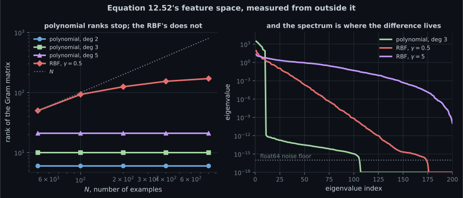
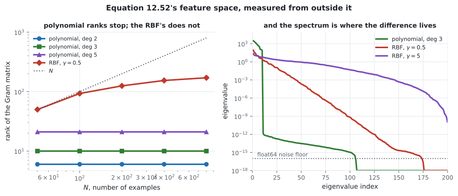
A kernel whose feature map has dimension $M$ has a Gram matrix of rank at most $M$, however many points you feed it. So watch the rank as $N$ grows:

rank_saturation.py

from scipy.special import comb
 
def k_rbf(A, B, gamma=0.5):
    d2 = ((A[:, None, :] - B[None, :, :]) ** 2).sum(-1)
    return np.exp(-gamma * d2)
 
rg = np.random.default_rng(3)
print(f"{'kernel':>24} {'C(D+p,p)':>10} {'N=50':>6} {'N=100':>7} "
      f"{'N=200':>7} {'N=400':>7} {'N=800':>7}")
for name, kf, fd in (
        ("polynomial, degree 2", lambda Z: k_poly(Z, Z, 2), int(comb(4, 2))),
        ("polynomial, degree 3", lambda Z: k_poly(Z, Z, 3), int(comb(5, 3))),
        ("polynomial, degree 5", lambda Z: k_poly(Z, Z, 5), int(comb(7, 5))),
        ("RBF, gamma = 0.5", lambda Z: k_rbf(Z, Z, 0.5), None),
        ("RBF, gamma = 5.0", lambda Z: k_rbf(Z, Z, 5.0), None)):
    rs = [int(np.linalg.matrix_rank(kf(rg.normal(0, 1, (n, 2)))))
          for n in (50, 100, 200, 400, 800)]     # numpy's default tolerance
    print(f"{name:>24} {str(fd) if fd else 'infinite':>10} "
          f"{rs[0]:>6} {rs[1]:>7} {rs[2]:>7} {rs[3]:>7} {rs[4]:>7}")

text

                  kernel   C(D+p,p)   N=50   N=100   N=200   N=400   N=800
    polynomial, degree 2          6      6       6       6       6       6
    polynomial, degree 3         10     10      10      10      10      10
    polynomial, degree 5         21     21      21      21      21      21
        RBF, gamma = 0.5   infinite     50      93     125     154     171
        RBF, gamma = 5.0   infinite     50     100     200     392     597

The polynomial rows are constant and equal to $\binom{D+p}{p}$ exactly. Eight hundred points in the plane cannot make a degree-3 polynomial kernel’s feature space bigger than ten dimensions — the data is irrelevant, the kernel decides.

The RBF rows never level off. That is what having no finite feature map looks like from the outside: no matter how many points you add, the Gram matrix keeps finding new directions.

The two RBF rows also say something the book does not: $\gamma$ controls how fast the feature space fills up. A narrow kernel ($\gamma = 5$) reaches full rank $N$ up to $N = 200$ and is still at $597$ of $800$; a wide one ($\gamma = 0.5$) is already down to $171$ of $800$, because its spectrum decays faster and most directions fall below floating-point resolution.

figure Equation 12.52's feature space, measured from outside it matplotlib

The cliff in the green curve is the polynomial's feature dimension. The RBF curves have no cliff — only decay — which is the difference between a finite feature space and one that is merely hard to reach.

Not every similarity function is a kernel

$$\forall \mathbf{z}\in\mathbb{R}^N : \mathbf{z}^\top\mathbf{K}\mathbf{z} \geq 0 \qquad \text{(12.53)}$$

Equation 12.53 requires every kernel matrix to be positive semidefinite. The frequently-used $\tanh(a\langle\mathbf{x},\mathbf{z}\rangle + c)$ “sigmoid kernel” is not:

function	smallest eigenvalue of $\mathbf{K}$	PSD?
linear	$-2.910\times10^{-14}$	yes
polynomial, degree $3$	$-5.336\times10^{-13}$	yes
RBF, $\gamma = 0.5$	$-1.049\times10^{-15}$	yes
$\tanh$	$\mathbf{-5.544\times10^{1}}$	no

Ten of its $120$ eigenvalues are negative, the most negative being $-55.44$. The first three rows are negative only at rounding level; the fourth is negative by fifty-five.

This matters beyond tidiness. Equation 12.41’s objective is $\tfrac12\boldsymbol\alpha^\top(\mathbf{Y}\mathbf{K}\mathbf{Y})\boldsymbol\alpha - \mathbf{1}^\top\boldsymbol\alpha$, and it is convex only when $\mathbf{K}$ is PSD. With a negative eigenvalue the dual is a non-convex quadratic, the duality guarantee of page 1206 no longer applies, and whatever the solver returns is not the solution to the problem Section 12.3 derived.

Figure 12.10, reproduced

Two concentric rings. No line in the plane separates them.

text

                    kernel   train acc   held-out acc   support vectors
                    linear      0.6417         0.6367               120
      polynomial, degree 2      1.0000         1.0000                 6
      polynomial, degree 3      1.0000         1.0000                 9
          RBF, gamma = 0.5      1.0000         1.0000                18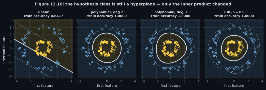

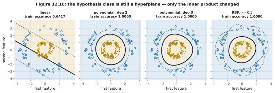
figure Figure 12.10: the hypothesis class is still a hyperplane — only the inner product changed matplotlib

The book's own caption makes the point: 'while the decision boundary is nonlinear, the underlying problem being solved is for a linear separating hyperplane.' The curve is a hyperplane in the feature space, seen from the input space.

The linear kernel gets $64\%$ and uses all $120$ examples as support vectors — a fit that has given up and is spending every multiplier. The degree-2 kernel gets everything right with six.

Why six is enough is worth spelling out, because it explains the whole section:

why_degree_two_suffices.py

rad2 = (XC ** 2).sum(1)                     # the squared radius of each point
print(f"squared radius, class +1 : [{rad2[YC > 0].min():.4f}, "
      f"{rad2[YC > 0].max():.4f}]")
print(f"squared radius, class -1 : [{rad2[YC < 0].min():.4f}, "
      f"{rad2[YC < 0].max():.4f}]")
print(f"separable on that single coordinate : "
      f"{bool(rad2[YC > 0].max() < rad2[YC < 0].min())}")

text

squared radius, class +1 : [0.2941, 2.1170]
squared radius, class -1 : [6.4572, 12.6957]
separable on that single coordinate : True

The two classes are separated by one derived feature, $x_1^2 + x_2^2$, and the degree-2 map contains $x_1^2$ and $x_2^2$ as two of its six coordinates. A threshold on their sum is a hyperplane in that space. The kernel never builds the space; it just computes the inner products as though it had.

Three different things called “kernel”

The book flags this, and it is worth repeating because all three appear in this module:

meaning	where	what it is
reproducing kernel	§12.4, here	a PSD similarity function with a hidden feature map
the null space	§2.7.3	$\{\mathbf{x} : \mathbf{A}\mathbf{x} = \mathbf{0}\}$
smoothing kernel	§11.5, page 1109	the bump placed on each point in density estimation

Page 1109’s KDE and this page’s SVM both put a Gaussian on every data point, and they are unrelated constructions that happen to share a word.

pch.quizTag Check your understanding

1. A Because the dual has fewer variables B Because in the dual the examples appear only through inner products with each other, never paired with a parameter — so a feature map changes nothing but that one matrix C Because the dual is convex D Because the primal has no inner products
   pch.quizShowAnswer

   B — Because in the dual the examples appear only through inner products with each other, never paired with a parameter — so a feature map changes nothing but that one matrix

2. A 800 B Approximately 400 C Exactly 10, which is C(D + p, p) — and it is 10 at N = 50, 100, 200, 400 and 800 alike D It depends on the data
   pch.quizShowAnswer

   C — Exactly 10, which is C(D + p, p) — and it is 10 at N = 50, 100, 200, 400 and 800 alike

3. A That the RBF feature space has about 171 dimensions B That the rank never saturates — unlike the polynomial rows it keeps climbing, which is what no finite feature map looks like from outside. The shortfall below N is the spectrum decaying past floating-point resolution C That the RBF is not a valid kernel D That the data was degenerate
   pch.quizShowAnswer

   B — That the rank never saturates — unlike the polynomial rows it keeps climbing, which is what no finite feature map looks like from outside. The shortfall below N is the spectrum decaying past floating-point resolution

4. A It only affects numerical precision B It makes the kernel matrix slower to compute C Equation 12.41's objective is convex only when K is positive semidefinite; with a negative eigenvalue the dual is a non-convex quadratic and the duality guarantee no longer applies D It means the feature space is infinite-dimensional
   pch.quizShowAnswer

   C — Equation 12.41's objective is convex only when K is positive semidefinite; with a negative eigenvalue the dual is a non-convex quadratic and the duality guarantee no longer applies

Exercises

Exercise 1 – Check that the kernel is an inner product

pch.exerciseTag pch.exerciseTitle

Exercise 2 – Watch a feature space saturate

pch.exerciseTag pch.exerciseTitle

Exercise 3 – Find a similarity function that is not a kernel

pch.exerciseTag pch.exerciseTitle

Recall card

• In the dual the examples appear only through their inner products with each other, never paired with a parameter, which is what makes a feature map cost one line.
• A kernel is a similarity function with a hidden feature map, and the kernel trick is using it without ever building that map.
• The explicit map of a degree-p polynomial has C(D + p, p) coordinates. At D equal to a thousand and degree five that is over eight trillion; the kernel is one inner product raised to a power.
• A feature space of dimension M gives a Gram matrix of rank at most M, which turns an invisible claim into a measurable one.
• Polynomial ranks saturate exactly. Degree two, three and five give rank 6, 10 and 21 at every N from 50 to 800 — the data cannot enlarge the feature space.
• The RBF’s rank never levels off, climbing from 50 to 171 as N goes from 50 to 800. That is what having no finite feature map looks like from outside.
• The bandwidth controls how fast the feature space fills. A narrow RBF reaches full rank up to N equal to 200 and 597 of 800; a wide one decays faster and reaches far less.
• Equation 12.53 is a requirement, not a convention. The dual’s objective is convex only when the kernel matrix is positive semidefinite.
• The tanh similarity function fails it, with ten negative eigenvalues and a smallest of minus 55.44, against roundoff-level negatives for the genuine kernels.
• Figure 12.10 reproduced: on two concentric rings a linear kernel reaches 64 percent and spends all 120 examples as support vectors, while a degree-2 kernel reaches 100 percent on six.
• Six suffices because the classes are separated by one derived feature, the squared radius, and the degree-2 map contains both squared coordinates.
• The decision boundary is curved and the hypothesis class is not. It is a hyperplane in the feature space, seen from the input space.
• Three unrelated things in this book are called a kernel: this one, the null space of Section 2.7.3, and the smoothing kernel of Section 11.5.

Next: Numerical Solution — §12.5, the subgradient of a loss that is not differentiable, and both SVMs written as standard quadratic programs.