
Finding Words for Intuitions
The book opens §1.1 with an unusual admission for a mathematics textbook: the words are slippery, and it is not going to fix that. Its exact position is that it “will not resolve the issue of ambiguity”, only make the context clear enough to survive.
That is worth taking seriously rather than skimming past. Machine learning inherited its vocabulary from statistics, from computer science, from optimisation and from neuroscience, and those fields did not coordinate. The result is that a sentence like “the algorithm learns a model from the data” contains three words with two or three meanings each — and the reason a paragraph sometimes refuses to make sense is not that the mathematics is hard, but that you picked the wrong meaning three sentences ago.
What you’ll learn
Section titled “What you’ll learn”- The three concepts at the core of machine learning, in the book’s own framing.
- Both senses of “machine learning algorithm”, and why conflating them makes §8.1 unreadable.
- The three ways to think about a vector, and which chapters use which.
- What “model” means when it is a function, and what it means when it is a distribution.
- Why “learning” and “memorising” are different, and what generalisation has to do with it.
Intuition: three concepts, and the arrow between them
Section titled “Intuition: three concepts, and the arrow between them”Machine learning is “designing algorithms that automatically extract valuable information from data”, and the emphasis the book puts on automatic is the whole point: the methods are meant to be general-purpose, working across many datasets without much domain-specific expertise being hand-coded into them.
  flowchart TD
  D["DATA
numerical, and treated as vectors"]
  M["MODEL
a simplified stand-in for the
unknown process that made the data"]
  L["LEARNING
optimise the parameters so the model
predicts the data well"]
  G["GENERALISATION
performs well on data it has never seen"]

  D --> M
  M --> L
  L --> G
  G -.->|"the actual goal"| M
  D -.->|"memorising this is easy
and worthless"| G
The dotted arrow from data to generalisation carries the warning. Performing well on data you have already seen “may only mean that we found a good way to memorise the data” — the book’s own phrasing. A lookup table scores perfectly on its training set and predicts nothing. Everything difficult in Chapter 8 exists to tell those two situations apart.
A real-life example: the estate agent
Section titled “A real-life example: the estate agent”You want to price a house. You have a spreadsheet of past sales — that is data. You assume price depends roughly linearly on floor area, bedroom count and distance to a station — that is a model, and notice it is an assumption, not something the data handed you. You tune the three coefficients until past sales are predicted well — that is learning.
Now the part that matters. You could instead memorise all 500 past sales exactly. Zero error on the spreadsheet, useless on the next house. The linear model is worse on the data you have and better on the data you want, and that trade is the subject of §8.2.
The math, and the words
Section titled “The math, and the words”“Algorithm” means two different things
Section titled ““Algorithm” means two different things”The book flags this one first because it causes the most confusion:
| sense | what it names | the book’s term |
|---|---|---|
| 1 | a system that makes predictions from input data | a predictor |
| 2 | a system that adapts internal parameters so the predictor does well on unseen input | training |
Both are routinely called “the machine learning algorithm”, in the same paper. Once you have the two names, sentences that were ambiguous become clear:
- “the algorithm is ” — almost always sense 2, the training cost.
- “the algorithm ran in 4 ms” — almost always sense 1, one prediction.
- “we compare three algorithms” — usually sense 1, three predictors, trained however.
There is a third sense the book mentions in passing and which trips people in Chapter 7: the numerical method inside the training procedure. “Gradient descent” is an algorithm; so is “linear regression”; so is “the fitted model”. Three levels, one word.
Data means vectors
Section titled “Data means vectors”The book is explicit and slightly brutal about this: while not all data is numerical, it assumes data “has already been appropriately converted into a numerical representation”, and from then on data is vectors.
That assumption hides an enormous amount of practical work — how you turn a sentence, an image or a category into numbers is most of applied machine learning — and the book sets it aside deliberately so it can be about the mathematics. Worth knowing that the boundary is a choice, not an oversight.
And then, as the book says, “as another illustration of how subtle words are”, vector itself has three readings:
| view | a vector is | who thinks this way | where it is used here |
|---|---|---|---|
| computer science | an array of numbers | programmers | §2.2, and all NumPy code |
| physics | an arrow with direction and magnitude | physicists, geometers | Chapter 3, all the p5 sketches |
| mathematics | any object that obeys addition and scaling | mathematicians | §2.4, the definition that matters |
The third is the one Chapter 2 actually adopts, and the payoff is surprising: because the definition demands only addition and scaling, polynomials are vectors, and so are audio signals, and so are functions. §3.7 computes the angle between two functions using exactly this, and it is not a metaphor — they satisfy the same axioms.
The three views are not competing. They are three faces of one object, and fluency means switching between them without noticing: an array for the code, an arrow for the intuition, an axiom-satisfier for the proof.
Model means two different things too
Section titled “Model means two different things too”A model is a simplified stand-in for the unknown process that generated the data — “a good model can then be used to predict what would happen in the real world without performing real-world experiments”. But it comes in two mathematical shapes:
- A function. . Feed it features, get a prediction. No uncertainty, and no way to express any.
- A distribution. . It describes how likely each pairing is, which lets you ask “how confident is this?” as a mathematical question rather than a vibe.
§8.1 develops both, and the choice determines almost everything downstream: least squares with a function view is an optimisation problem, and least squares with a distribution view is maximum likelihood under Gaussian noise (§9.1). Same estimator, two stories — and only the second one tells you where the error bars come from.
Learning means two different things
Section titled “Learning means two different things”Training the model means using the data to optimise some parameters against a utility function that scores how well the model predicts. The book gives the analogy directly: most training methods are “analogous to climbing a hill to reach its peak”, where the peak is the maximum of the performance measure. Chapter 7 is that hill-climb, done properly, and Chapter 5 supplies the gradient that tells you which way is up.
The second sense of learning is non-parametric: some methods have nothing to optimise, and “learn” by keeping the data. -nearest-neighbours is the standard example — training is storing the dataset. Both are called learning; only one involves a hill.
The three bullets the whole book reduces to
Section titled “The three bullets the whole book reduces to”The book closes §1.1 by compressing itself into three lines, and they are worth memorising because each one names the chapters that deliver it:
- We represent data as vectors. — Chapters 2, 3, 4.
- We choose an appropriate model, using either the probabilistic or the optimisation view. — Chapters 6, 8.
- We learn from available data by numerical optimisation, aiming to do well on data not used for training. — Chapters 5, 7, 8.
Every remaining page in this module serves one of those three sentences.
Worked example: one sentence, eight readings
Section titled “Worked example: one sentence, eight readings”Take the sentence
“The algorithm learns a model from the data.”
and count the readings. Two senses of “algorithm”, two of “model”, two of “learn” — eight combinations, of which these four are ones people actually mean:
| algorithm | model | learn | what the sentence then means |
|---|---|---|---|
| training procedure | function | optimise parameters | gradient descent fits the weights of a network |
| training procedure | distribution | optimise parameters | maximum likelihood fits a Gaussian’s mean and variance |
| predictor | function | store data | a nearest-neighbour classifier keeps the training set |
| numerical method | function | optimise parameters | L-BFGS minimises a logistic-regression objective |
The other four are combinations nobody intends but a reader can accidentally construct. That is the failure mode: not misunderstanding the mathematics, but silently choosing reading 3 while the author meant reading 1.
The habit that fixes it: when a sentence stops making sense, do not reread it harder. Substitute the specific term — predictor, training procedure, numerical method — and see which substitution makes the sentence true. Usually only one does.
See it move
Section titled “See it move”One dataset, three framings. Drag the framing knob and watch the same eight points get re-described: as an array of numbers, as arrows from the origin, and as a fitted model with residuals. Nothing about the data changes — only what you are being asked to see.
The third framing is the one to sit with. Dragging and to shrink the sum of squared residuals is learning, done by hand — and the hill-climbing analogy the book uses is exactly what your hand is doing. Chapter 7 replaces your hand with a gradient.
From scratch
Section titled “From scratch”The three views of a vector, and hand-rolled “learning”, in one script.
import numpy as np

X = np.array([0.4, 0.9, 1.3, 1.7, 2.2, 2.6, 3.0, 3.4])
Y = np.array([0.7, 0.9, 1.4, 1.3, 1.9, 1.8, 2.5, 2.4])
rows = np.c_[X, Y]

# ---- view 1: an array of numbers (computer science) ----
print("shape:", rows.shape, " dtype:", rows.dtype, " row 3:", rows[3])

# ---- view 2: arrows with length and direction (physics) ----
lengths = np.linalg.norm(rows, axis=1)
angles = np.degrees(np.arctan2(rows[:, 1], rows[:, 0]))
print("lengths:", np.round(lengths, 3))
print("angles :", np.round(angles, 1))

# ---- view 3: objects obeying addition and scaling (mathematics) ----
# The axioms do not mention numbers, so POLYNOMIALS are vectors too.
p = np.array([1.0, -2.0, 0.5])        # 1 - 2t + 0.5t^2, as coefficients
q = np.array([0.0,  3.0, 1.0])        #     3t +   1t^2
print("p + q is a polynomial:", p + q)
print("3p is a polynomial   :", 3 * p)

# ---- 'learning', by hand then properly ----
def sse(w, b):
    return float(((Y - (b + w * X)) ** 2).sum())

print("\nsse at w=0.62, b=0.35:", round(sse(0.62, 0.35), 4))
print("sse at w=0.55, b=0.40:", round(sse(0.55, 0.40), 4))

# The optimum, by least squares — Chapter 9 derives this formula.
A = np.c_[np.ones_like(X), X]
b_opt, w_opt = np.linalg.lstsq(A, Y, rcond=None)[0]
print("best b, w           :", round(b_opt, 4), round(w_opt, 4))
print("sse at the optimum  :", round(sse(w_opt, b_opt), 4))

# ---- memorising is not learning ----
# A lookup table is perfect on the training data and undefined off it.
table = dict(zip(X, Y))
print("\nlookup on a seen point   :", table[X[2]])
print("lookup on an unseen point:", table.get(1.5, "no idea"))
print("model on that same point :", round(b_opt + w_opt * 1.5, 4))shape: (8, 2) dtype: float64 row 3: [1.7 1.3]
lengths: [0.806 1.273 1.91 2.14 2.907 3.162 3.905 4.162]
angles : [60.3 45. 47.1 37.4 40.8 34.7 39.8 35.2]
p + q is a polynomial: [1. 1. 1.5]
3p is a polynomial : [ 3. -6. 1.5]
sse at w=0.62, b=0.35: 0.2291
sse at w=0.55, b=0.40: 0.3933
best b, w : 0.4402 0.6051
sse at the optimum : 0.1974
lookup on a seen point : 1.4
lookup on an unseen point: no idea
model on that same point : 1.3478The last three lines are the point of Chapter 8 in miniature. The lookup table is perfect on every point it has seen and has literally nothing to say about . The fitted line is imperfect everywhere and answers anyway. Only one of those is a model.
Note the two hand guesses. w=0.62, b=0.35 scores ; nudging to w=0.55, b=0.40 makes it
worse, at — so hand-tuning is not even reliably monotone. The true optimum is
w=0.6051, b=0.4402, scoring . Hand-tuning gets in the neighbourhood and cannot get to the
bottom, which is the argument for Chapter 7.
On real data
Section titled “On real data”The three ambiguities on this page are not merely verbal. Each one has a measurable consequence, and these figures are those measurements.
Reading the plot
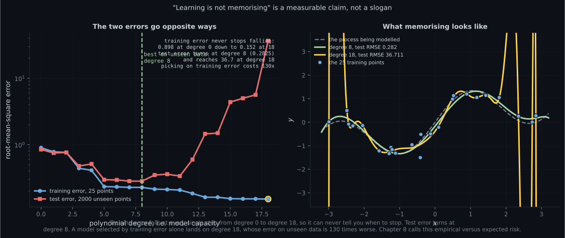
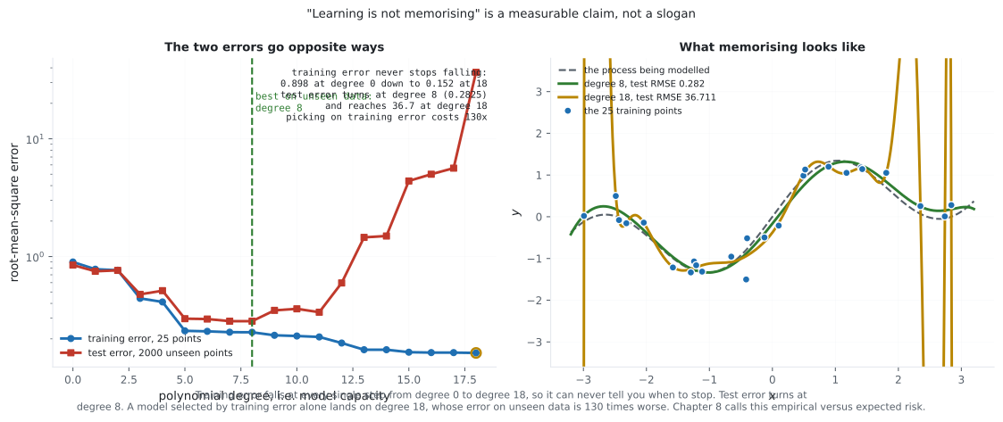
Section titled “Reading the plot”The first figure is the caution box above, in numbers. Look at the blue curve first and note what it never does: it never turns. Training error falls from at degree to at degree , monotonically, at every step. There is no kink, no elbow, nothing in its shape that says “stop here”. If training performance is your only instrument, the honest reading of that curve is “keep adding capacity”, and it will be the honest reading no matter how far you extend the axis. The red curve is the same models scored on points they never saw: it bottoms out at degree with an error of and then leaves, reaching by degree — a factor of . The right panel shows what the two chosen models look like. The degree- curve threads closer to the training points than the degree- curve does, which is exactly why training error prefers it, and between the points it swings to values the process never produces.
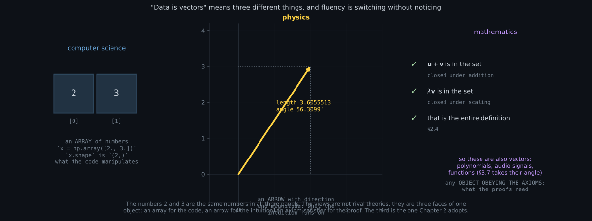
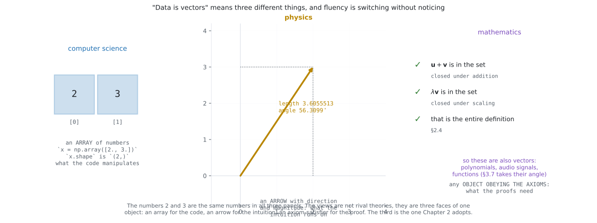
The second figure has no measurement to make, and that is the point. The pair is one
object. As an array it has a shape and an index order and is the thing NumPy multiplies. As an arrow
it has length and angle , which is what makes “orthogonal” and “projection” mean
anything. As an element of a vector space it has only two properties — you can add two of them and you
can scale one — and that is the definition §2.4 adopts. The reason to prefer the thinnest definition
is on the right of the panel: because it demands so little, things that are not lists of numbers
satisfy it too. Polynomials do. Audio signals do. Functions do, which is why §3.7 can compute the
angle between and and get a real answer rather than a metaphor.
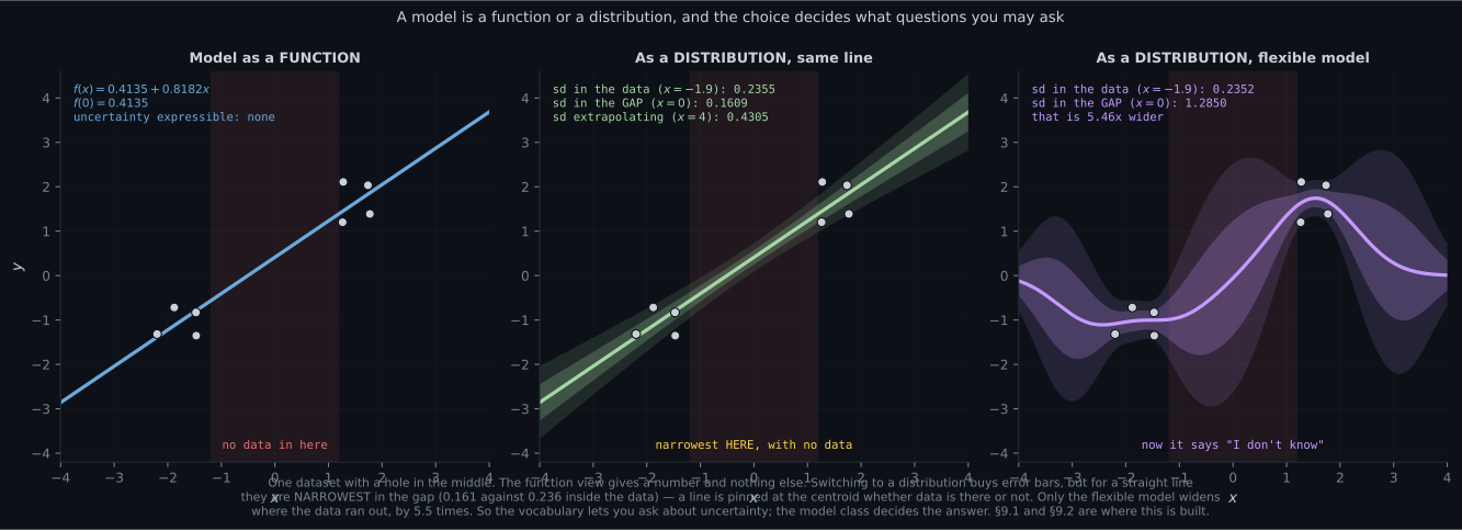
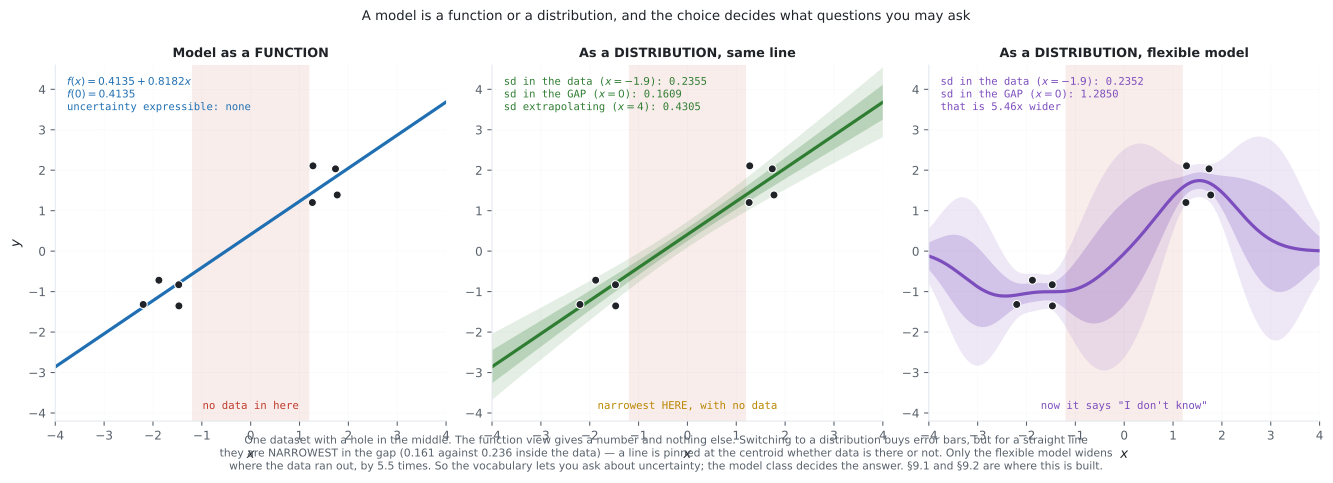
The third figure corrects a claim that is usually made too strongly. All three panels fit the same eight points, which have a deliberate hole between and . The left panel is the function view: it returns and has no vocabulary in which to say how much to trust it. The middle panel switches to the distribution view without changing the model — still a straight line — and now there is a band. But read the band carefully, because it does not do what the slogan promises. Inside the data the standard deviation is ; in the empty middle it is , which is narrower. That is not a bug. A straight line is pinned most tightly near the centroid of its inputs, and the centroid of this dataset sits in the middle of the gap. The model is confident there because a line has nowhere else to go, not because it has evidence.
The right panel changes the model class, keeping the distribution view: fourteen basis functions instead of two. Inside the data its standard deviation is , statistically the same as the line’s — where there is evidence, the two agree. Across the gap it reaches , some times wider. That is a model saying it does not know. So the sense of “model” you pick decides whether the question “how confident are you?” is expressible at all, and the model class you pick decides whether the answer is any good. Confusing those two is how a confidently wrong extrapolation gets shipped.
Pitfalls
Section titled “Pitfalls”Compare
Section titled “Compare”| word | sense A | sense B | how to tell |
|---|---|---|---|
| algorithm | the predictor | the training procedure | does the sentence talk about a prediction, or about fitting? |
| model | a function | a distribution | is uncertainty being expressed? |
| learning | optimise parameters | store the data | is there anything to optimise? |
| vector | array, or arrow | an object obeying the axioms | is a proof being made, or a computation? |
| training data | the fitting sample | occasionally, everything not held out | is a validation split mentioned? |
-
The book says the phrase machine learning algorithm is used in at least two senses. What are they?
The first is what the book calls a predictor; the second is training. Section 8.1 gives each its own mathematics, so collapsing them makes that section unreadable.
pch.quizShowAnswer
B — A system that makes predictions, and a system that adapts the predictor's parameters — The first is what the book calls a predictor; the second is training. Section 8.1 gives each its own mathematics, so collapsing them makes that section unreadable.
-
Why does the mathematical definition of a vector matter more than the array or arrow pictures?
The axioms mention nothing about components, so anything satisfying them is a vector. That is what lets section 3.7 compute the angle between two functions — not as an analogy, but as the same operation.
pch.quizShowAnswer
B — Because it only demands addition and scaling, it admits polynomials, audio signals and functions as vectors — The axioms mention nothing about components, so anything satisfying them is a vector. That is what lets section 3.7 compute the angle between two functions — not as an analogy, but as the same operation.
-
A model scores zero error on its training set. What does that tell you?
The book raises exactly this on its second page. A lookup table achieves zero training error and predicts nothing. Empirical risk and expected risk are different quantities, which is what section 8.2 is about.
pch.quizShowAnswer
B — Very little on its own — it may simply have memorised the training data — The book raises exactly this on its second page. A lookup table achieves zero training error and predicts nothing. Empirical risk and expected risk are different quantities, which is what section 8.2 is about.
-
What is the practical difference between treating a model as a function and treating it as a distribution?
They can agree exactly on the point prediction — least squares is both an optimisation problem and maximum likelihood under Gaussian noise — but only the distribution view says how confident the prediction is.
pch.quizShowAnswer
B — The distribution view can express uncertainty, so it can produce error bars where the function view cannot — They can agree exactly on the point prediction — least squares is both an optimisation problem and maximum likelihood under Gaussian noise — but only the distribution view says how confident the prediction is.
🧪 Try It Yourself
Section titled “🧪 Try It Yourself”Exercise 1 – Data as an array
Section titled “Exercise 1 – Data as an array”Exercise 2 – The same data as arrows
Section titled “Exercise 2 – The same data as arrows”Exercise 3 – Polynomials really are vectors
Section titled “Exercise 3 – Polynomials really are vectors”Exercise 4 – Learning by hand, then properly
Section titled “Exercise 4 – Learning by hand, then properly”Exercise 5 – Memorising is not learning
Section titled “Exercise 5 – Memorising is not learning”Recall card
Section titled “Recall card”- The book will not resolve the ambiguity in machine learning’s vocabulary; it only promises to make the context clear. Knowing which words are overloaded is the reader’s job.
- “Machine learning algorithm” has two senses — a predictor that makes predictions, and training, which adapts the predictor’s parameters. Section 8.1 treats them as separate phases.
- There is a third sense of algorithm: the numerical method inside the training procedure, like gradient descent.
- Data as vectors is an assumption, stated once and never revisited — converting text, images and categories into numbers is outside the book’s scope, not trivial.
- A vector has three readings — an array (computer science), an arrow with direction and magnitude (physics), and any object obeying addition and scaling (mathematics).
- The mathematical reading is the one that pays, because it admits polynomials, audio signals and functions as vectors, which is what makes section 3.7’s angle between two functions literal rather than metaphorical.
- A model is either a function or a distribution, and only the distribution view can express uncertainty — the reason Bayesian linear regression has error bars and maximum likelihood does not.
- Learning means optimising parameters, or simply storing the data — parametric versus non-parametric, and only the first involves the hill-climb.
- Training performance alone tells you nothing, because doing well on seen data may just mean the model memorised it. Generalisation to unseen data is the actual goal.
- The whole book reduces to three bullets — represent data as vectors, choose a model in the probabilistic or optimisation view, and learn by numerical optimisation aiming at unseen data.
Next: the two routes through the material, and the map of what depends on what — Two Ways to Read This Book.
pch.coffeeTagline
pch.coffeeCtapch.feedbackHeading
pch.feedbackSubheading