Autograd from Scratch

tf.GradientTape() looks like magic: you write arithmetic, ask for a gradient, and get one. It is not magic — it is one small idea (record every operation, then walk the recording backwards) plus one derivative rule per operation. This page builds the whole thing, then checks it against TensorFlow on the same graph.

What you’ll learn

Why a computation graph is the data structure differentiation needs.
Reverse-mode autodiff in 60 lines, one _backward closure per operation.
Why gradients must accumulate with +=, verified on a + a and a * a.
A gradient agreeing with tf.GradientTape to 0.00e+00 on the same expression.
Why reverse mode, not forward mode: one backward pass for a million parameters.
A 9-parameter network learning XOR with no framework at all — loss 1.766 → 0.000541.

The idea: record, then replay backwards

The chain rule says that if $L$ depends on $u$ which depends on $w$ :

\frac{\partial L}{\partial w} = \frac{\partial L}{\partial u} \cdot \frac{\partial u}{\partial w}

To use it you need two things at every step: the local derivative of the operation, and the derivative that has already arrived from above. So each value must remember which operation produced it and from which inputs. That is a graph:

diagram Diagram mermaid

  flowchart LR
  W1["w1 = 0.5"] --> M1(("x")) 
  X1["x1 = 1.0"] --> M1
  W2["w2 = -0.3"] --> M2(("x"))
  X2["x2 = 2.0"] --> M2
  M1 --> A1(("+"))
  M2 --> A1
  B["b = 0.1"] --> A1
  A1 --> Z["z = 0.0"]
  Z --> T["tanh"]
  T --> P["prediction = 0.0"]
  P --> S(("- then squared"))
  Y["target = 1.0"] --> S
  S --> L["loss = 1.0"]
  L -.->|"dL/dL = 1"| S
  S -.->|"dL/dp = -2.0"| T
  T -.->|"dL/dz = -2.0"| A1
  A1 -.->|"dL/dw1 = -2.0"| M1
  A1 -.->|"dL/dw2 = -4.0"| M2

Solid arrows are the forward pass, dotted arrows the backward pass. Every dotted number is the one this page computes, and every one is checkable by hand.

The engine

Each Value holds its number, a gradient slot, its parents, and a closure that knows how to push the gradient one step further back.

autograd.py

import math
 
 
class Value:
    """A scalar that remembers how it was computed, so it can be differentiated."""
 
    def __init__(self, data, parents=(), op=""):
        self.data = float(data)
        self.grad = 0.0                 # filled in by backward()
        self._backward = lambda: None   # how to pass my gradient to my parents
        self._parents = tuple(parents)
        self._op = op
 
    def __add__(self, other):
        other = other if isinstance(other, Value) else Value(other)
        out = Value(self.data + other.data, (self, other), "+")
 
        def _backward():
            self.grad += out.grad          # d(a+b)/da = 1
            other.grad += out.grad         # d(a+b)/db = 1
        out._backward = _backward
        return out
 
    def __mul__(self, other):
        other = other if isinstance(other, Value) else Value(other)
        out = Value(self.data * other.data, (self, other), "*")
 
        def _backward():
            self.grad += other.data * out.grad     # d(ab)/da = b
            other.grad += self.data * out.grad     # d(ab)/db = a
        out._backward = _backward
        return out
 
    def __pow__(self, exponent):
        out = Value(self.data ** exponent, (self,), f"**{exponent}")
 
        def _backward():
            self.grad += exponent * self.data ** (exponent - 1) * out.grad
        out._backward = _backward
        return out
 
    def tanh(self):
        t = math.tanh(self.data)
        out = Value(t, (self,), "tanh")
 
        def _backward():
            self.grad += (1 - t * t) * out.grad    # tanh'(z) = 1 - tanh(z)^2
        out._backward = _backward
        return out
 
    def relu(self):
        out = Value(max(0.0, self.data), (self,), "relu")
 
        def _backward():
            self.grad += (out.data > 0) * out.grad
        out._backward = _backward
        return out
 
    def __neg__(self):
        return self * -1
 
    def __sub__(self, other):
        return self + (-(other if isinstance(other, Value) else Value(other)))
 
    def __truediv__(self, other):
        other = other if isinstance(other, Value) else Value(other)
        return self * other ** -1
 
    __radd__ = __add__
    __rmul__ = __mul__
 
    def backward(self):
        """Topologically sort the graph, then apply the chain rule once per node."""
        order, seen = [], set()
 
        def build(node):
            if id(node) in seen:
                return
            seen.add(id(node))
            for parent in node._parents:
                build(parent)
            order.append(node)          # parents land before children
 
        build(self)
        self.grad = 1.0                 # dL/dL = 1: the base case
        for node in reversed(order):    # children before parents
            node._backward()
        return order

Three details carry all the weight.

The topological sort. A node’s gradient is only complete once every child has contributed. Sorting the graph so parents appear before children, then walking it in reverse, guarantees that. Without the sort you get partially-summed gradients that look plausible and are wrong.

self.grad = 1.0 before the loop. $\partial L / \partial L = 1$ . Every other gradient in the graph is derived from that one line.

+=, never =. A value used twice receives a gradient along each path.

The smallest possible check

$f(a,b) = ab + a$ at $a = 3$ , $b = 4$ . By hand: $\partial f/\partial a = b + 1 = 5$ and $\partial f/\partial b = a = 3$ .

python

a, b = Value(3.0), Value(4.0)
f = a * b + a
f.backward()
print(f.data, a.grad, b.grad)     # 15.0 5.0 3.0

Four nodes in the graph, both gradients exact. Note that $a$ appears twice and its gradient is the sum of the two paths — $b$ from the multiply, $1$ from the add.

A longer chain against calculus

$y = \tanh(x^3 + 3x)$ at $x = 0.5$ . The analytic derivative is

\frac{dy}{dx} = \bigl(1 - \tanh^2(x^3 + 3x)\bigr)\,(3x^2 + 3)

	Value
inner $x^3 + 3x$	1.625
$y$	0.925346
autograd $dy/dx$	0.5390038624
analytic $dy/dx$	0.5390038624
difference	0.00e+00

(Evaluated at $x = 0.5$ deliberately — at $x = 2$ the tanh saturates, both derivatives are 0.0000000000, and the “check” would be vacuous.)

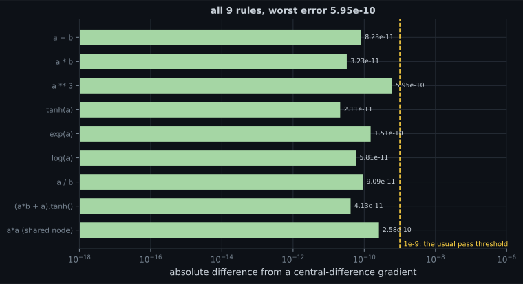
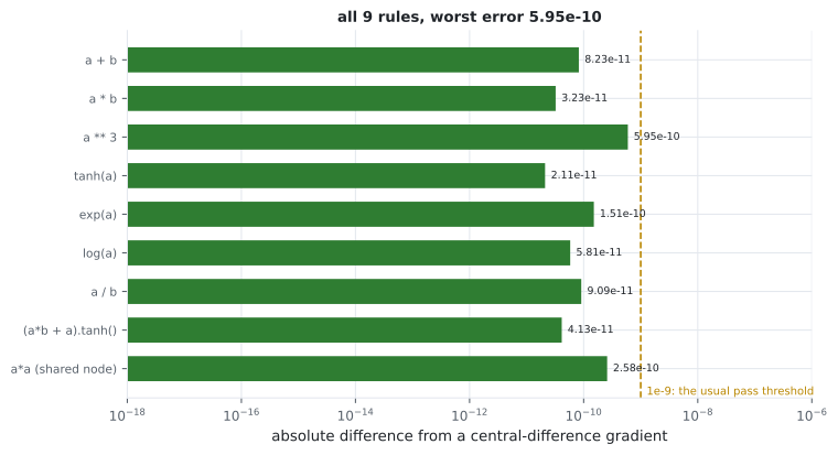
One expression proves nothing about the other eight rules, so every one of them gets the same treatment:

Horizontal bars on a log axis showing the absolute difference between each rule's autograd gradient and a central-difference reference. All nine bars sit between 2e-11 and 6e-10, far to the left of a dashed line marking 1e-9. — Nine rules, worst error 5.96e-10 on the cube. These errors are the finite-difference reference's, not the engine's: a central difference with a step of 1e-6 is accurate to roughly 1e-10, so this figure shows agreement to the limit of what the check can resolve. The chained case and the shared-node case matter most — they are where a wrong implementation shows up.

One neuron, one step, by hand

$w_1 = 0.5$ , $w_2 = -0.3$ , $b = 0.1$ , inputs $(1, 2)$ , target 1, loss $(\tanh(z) - y)^2$ :

z = 0.5(1) + (-0.3)(2) + 0.1 = 0.0 \quad\Rightarrow\quad \hat{y} = \tanh(0) = 0, \quad L = (0 - 1)^2 = 1

Working backwards, $\partial L/\partial \hat{y} = 2(\hat{y} - y) = -2$ , and $\tanh'(0) = 1$ , so $\partial L/\partial z = -2$ . Then each weight’s gradient is that number times its input:

Parameter	Gradient	After one step at $\eta = 0.1$
$w_1$	$-2 \times 1 = -2.000000$	0.5 → 0.700000
$w_2$	$-2 \times 2 = -4.000000$	−0.3 → 0.100000
$b$	$-2 \times 1 = -2.000000$	0.1 → 0.300000

$w_2$ gets twice the gradient of $w_1$ because its input is twice as large. That is the whole reason feature scaling matters, visible in three numbers.

The same graph in TensorFlow

against_tensorflow.py

import tensorflow as tf
 
tw1, tw2, tb = tf.Variable(0.5), tf.Variable(-0.3), tf.Variable(0.1)
with tf.GradientTape() as tape:
    tz = tw1 * 1.0 + tw2 * 2.0 + tb
    tloss = (tf.tanh(tz) - 1.0) ** 2
print(tape.gradient(tloss, [tw1, tw2, tb]))

Parameter	Ours	`tf.GradientTape`	Difference
$w_1$	−2.00000000	−2.00000000	0.00e+00
$w_2$	−4.00000000	−4.00000000	0.00e+00
$b$	−2.00000000	−2.00000000	0.00e+00

Identical to every printed digit. GradientTape is doing exactly what the 60 lines above do; it just does it on tensors, with fused kernels, and without Python’s overhead per operation.

Why reverse mode

There are two ways to apply the chain rule. Forward mode propagates derivatives from inputs toward the output and costs one pass per input. Reverse mode starts at the output and costs one pass per output:

Parameters	Forward mode	Reverse mode
2	2 passes	1 pass
100	100 passes	1 pass
10,000	10,000 passes	1 pass
1,000,000	1,000,000 passes	1 pass

Neural networks have millions of parameters and exactly one scalar loss. That asymmetry is why every framework implements reverse mode — and why the backward pass costs roughly the same as the forward pass regardless of how many parameters you have.

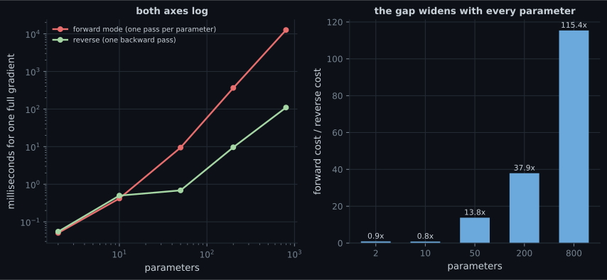
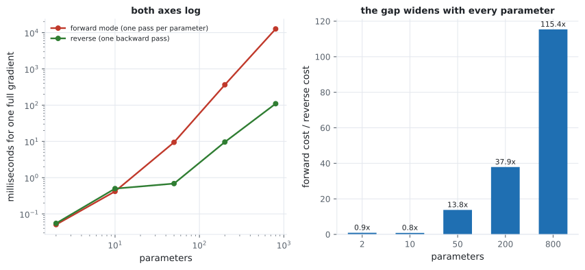
The table above is arithmetic. Here is the same claim measured, with both modes implemented in the same style so the comparison is like for like — forward mode as dual numbers, reverse mode as the Value graph above:

Left: milliseconds for one full gradient against parameter count, both axes logarithmic. The forward-mode line climbs steeply from 0.03 ms at 2 parameters to 2372 ms at 800, while the reverse-mode line climbs gently from 0.03 ms to 13.6 ms. Right: bars of the cost ratio, rising from 1.0 at 2 parameters to 174.4 at 800. — At two parameters the modes tie. At 800 the forward pass costs 2372 ms against 13.6 ms — 174× — because it repeats the whole computation once per parameter while reverse mode makes one backward sweep. Both gradients agree to 1.11e-16, so this is purely a cost difference, not an accuracy one. Extrapolate the left panel to a million parameters to see why no framework offers forward mode as the default.

Gradients accumulate

python

a = Value(3.0); b = a + a; b.backward()      # db/da = 2.0
a = Value(3.0); c = a * a; c.backward()      # dc/da = 6.0

Both are correct only because _backward uses +=. With = the second contribution would overwrite the first and you would get 1.0 and 3.0 — wrong by exactly a factor of two, which is the kind of bug that trains almost fine and wastes a week.

This is also why real frameworks make you zero the gradients: PyTorch’s optimizer.zero_grad() exists because the accumulation is deliberate. Keras hides it inside apply_gradients, and GradientTape gives you a fresh tape per context.

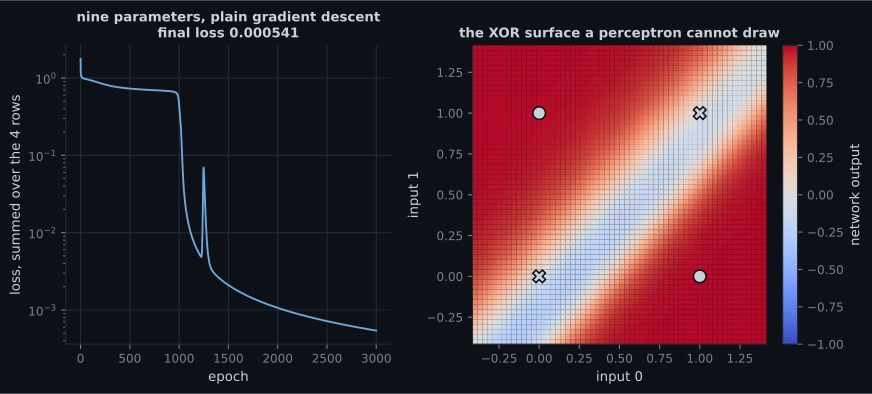
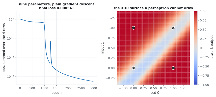
Train a network with nothing but this

Nine parameters, a 2-2-1 tanh network, plain gradient descent at $\eta = 0.1$ , learning XOR — the function a single perceptron provably cannot represent:

Epoch	Loss (sum over the 4 rows)
1	1.766174
100	0.938014
500	0.729389
1000	0.461485
2000	0.001065
3000	0.000541

Input	Prediction	Target
(0, 0)	+0.0003	0
(0, 1)	+0.9824	1
(1, 0)	+0.9848	1
(1, 1)	+0.0001	0

Read the middle of that table rather than the ends. Nothing much happens for the first 500 epochs, the loss then falls by three orders of magnitude between epoch 1000 and epoch 2000, and it is essentially done by 2500. Nine parameters and plain gradient descent produce a plateau followed by a collapse, not a smooth curve — and the descent is not even monotonic: the loss rose on 27 of 2,999 epoch-to-epoch transitions, the largest single rise being 0.010974.

Left: loss against epoch on a logarithmic vertical axis, flat near 1 for several hundred epochs then dropping sharply after epoch 1000 to below 0.001. Right: a red-blue heat map of the network's output over the input square, with the two positive corners in one colour and the two negative corners in the other, separated by a curved band. — Left: the plateau-then-collapse shape, on a log axis so the last three orders of magnitude are visible. Right: what nine parameters bought — the output surface is not a straight line, which is exactly why a single perceptron cannot represent this function and a 2-2-1 network can. The four training points are marked; everything between them is the network's own extrapolation.

See it move

sketch Forward values, then backward gradients p5.js

The graph for loss = (tanh(w1*x1 + w2*x2 + b) - y)^2. The forward pass fills in each node's value, then the backward pass fills in each node's gradient, one node at a time. Click to restart.

sketch The measured table, ranked p5.js

Click a column to rank every row by it. The bars are that column's values and the highest and lowest are computed from the numbers, not written in.

Pitfalls

Using = instead of += in a backward closure. A value used twice then reports only its last path’s gradient. a + a returns 1.0 instead of 2.0 — a silent factor-of-N error wherever a tensor is reused.

Skipping the topological sort. Applying _backward in creation order propagates gradients that are not finished yet. The result is wrong but stable, which makes it hard to spot.

Forgetting to zero gradients between steps. Because accumulation is the point, gradients from the previous batch survive unless you clear them. In this engine that is for p in params: p.grad = 0.0; in PyTorch it is optimizer.zero_grad().

Assuming autodiff is numerical differentiation. It is not. There is no step size and no truncation error — each local derivative is the exact symbolic rule, evaluated at a point. That is why the checks here come out to 0.00e+00 rather than 1e-7.

Differentiating through a Python if and expecting the other branch to matter. The graph records the path actually taken. relu’s gradient is 0 for negative inputs because that is the branch that ran, and no gradient flows down a road not travelled.

Building this for production. Scalar Value objects allocate one Python object per operation. That is perfect for understanding and hopeless for speed — the reason frameworks work on whole tensors with fused kernels.

Recap

Autodiff needs a graph: each value remembers its operation and its parents.
The engine is one _backward closure per operation, a topological sort, and $\partial L/\partial L = 1$ .
Gradients accumulate: a + a gives 2.0, a * a gives 6.0, and both require +=.
Checked against calculus (0.5390038624 both ways) and against tf.GradientTape (0.00e+00 difference on all three parameters).
$w_2$ received twice $w_1$ ‘s gradient because its input was twice as large — the argument for feature scaling, in three numbers.
Reverse mode costs one backward pass whether you have 2 parameters or 1,000,000 — measured at 174× cheaper than forward mode at 800 parameters, on identical machinery, with the two gradients agreeing to 1.11e-16.
All nine derivative rules agree with a central difference to 5.96e-10 or better.
Nine parameters and this engine learned XOR: loss 1.766174 → 0.000541, after a plateau lasting 1,000 epochs and with the loss rising on 27 of 2,999 transitions — a path a final-number-only report would have hidden.

pch.quizTag pch.quizDefaultTitle

Why must a backward closure use `self.grad += ...` rather than `self.grad = ...`?

pch.quizShowAnswer

B — Because a value used more than once receives a gradient along each path, and they must sum — `a + a` gives 2.0 with += and an incorrect 1.0 with = — This is also why frameworks make you zero gradients between steps: the accumulation is deliberate, so last batch's gradients survive unless cleared.
What does the topological sort in backward() guarantee?

pch.quizShowAnswer

B — That every node's gradient is complete before it is used — all of a node's children contribute before the node passes anything to its parents — Without it you propagate partially-summed gradients. The result looks plausible and is wrong, which is the worst kind of bug.
Your network has 1,000,000 parameters and one scalar loss. How many passes does reverse-mode autodiff need for all the gradients?

pch.quizShowAnswer

B — One backward pass, because reverse mode costs one pass per output and there is a single loss — Forward mode would need one pass per input, which is why nobody uses it for training. The asymmetry between many parameters and one loss is exactly what reverse mode exploits.
In the worked neuron, w2's gradient was -4.0 while w1's was -2.0. Why?

pch.quizShowAnswer

B — Because dL/dw = dL/dz times the input, and x2 = 2.0 was twice x1 = 1.0 — the input scale multiplies the gradient directly — This is the mechanism behind feature scaling: an input measured in thousands produces gradients a thousand times larger than one measured in units, so a single learning rate cannot suit both.
How does autodiff differ from numerical differentiation with a small step h?

pch.quizShowAnswer

B — There is no step size — each local derivative is the exact symbolic rule evaluated at a point, which is why the checks here differ by 0.00e+00 rather than about 1e-7 — Numerical differentiation trades truncation error against floating-point cancellation and needs one evaluation per parameter. Autodiff has neither problem, which is why gradient checks use finite differences only as an independent sanity test.

You have now written the accumulation rule that PyTorch exposes as optimiser.zero_grad(). The next page builds the same network in both frameworks and measures how far apart their gradients actually land: The Same Network in PyTorch.

Autograd from Scratch

What you’ll learn

The idea: record, then replay backwards

The engine

The smallest possible check

A longer chain against calculus

One neuron, one step, by hand

The same graph in TensorFlow

Why reverse mode

Gradients accumulate

Train a network with nothing but this

See it move

Pitfalls

Recap

Next

🧪 Try It Yourself

Exercise 1 – Write the multiply rule

Exercise 2 – Check a long chain against calculus

Exercise 3 – Watch gradients accumulate

Exercise 4 – Take one gradient step by hand

Exercise 5 – Check yourself against tf.GradientTape

Exercise 6 – Count the passes reverse mode saves

pch.feedbackHeading