
Phase 1 - Neural Network Foundations
Every architecture in this module — convolutional networks, recurrent networks, Transformers, diffusion models — is neurons, layers and activation functions arranged differently, trained by the same update rule. Phase 1 builds that base, and it does so by measuring rather than asserting: every number on every page in this phase came from code that ran on a CPU laptop, and several of them contradict what tutorials usually claim.
What this phase covers
Section titled “What this phase covers”flowchart LR A["401.5 Tensors
rank, shape, broadcasting"] --> B["402 Perceptron
one neuron, one line"] B --> C["403 MLP
hidden layers"] C --> D["404 Activations
ReLU, sigmoid, softmax"] D --> E["405 Keras APIs
Sequential, Functional, subclassing"] E --> F["405.5 Gradient descent
the update rule and its limits"] F --> G["405.7 Autograd from scratch
60 lines, no framework"] G --> T["405.9 The same net in PyTorch
same maths, different defaults"] G --> H["406 IMDB
binary"] H --> I["407 Reuters
multiclass"] I --> J["408 House prices
regression"] J --> K["Phase 2:
making depth trainable"]
Read them in order. Each page assumes the previous one, and the three worked examples at the end reuse everything before them.
The ten pages, and what each one proves
Section titled “The ten pages, and what each one proves”| # | Page | The result it delivers |
|---|---|---|
| 401.5 | Tensors and Tensor Operations | Rank, shape and dtype; the broadcasting rule and its failure modes; why matmul costs flops — and the measured surprise that float16 can be hundreds of times slower than float32 on a CPU |
| 402 | Introduction to Neural Networks (The Perceptron) | The perceptron learning rule, the proof it cannot learn XOR, and a nine-parameter two-layer fix worked out by hand |
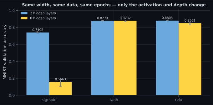
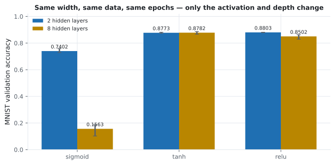
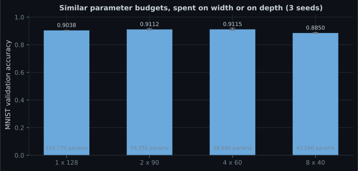
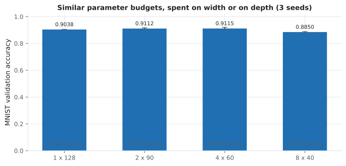
| 403 | Multi-Layer Perceptron (MLP) | What a hidden layer actually buys: 0.68 → 0.97 on the same classifier, plus width against depth at a fixed parameter budget |
| 404 | Activation Functions | Why a network without activations collapses to one linear layer, and what each activation’s derivative costs at depth |
| 405 | Building Networks with Keras | Three APIs producing bit-identical models, and four stopping policies spanning 2.8941 to 2.7653 test MAE |
| 405.5 | How Neural Networks Learn | The update rule verified to 0.00e+00 against Keras, the stability limit derived and tested, and a learning-rate sweep from 0.1320 to 0.8960 accuracy |
| 405.7 | Autograd from Scratch | Reverse-mode automatic differentiation in about 60 lines, matching tf.GradientTape to the last digit |
| 405.9 | The Same Network in PyTorch | Identical weights give gradients agreeing to 7.45e-09; identical training gives 0.8990 both ways; the real gaps are the defaults |
| 406 | Classifying Movie Reviews (IMDB) | Binary classification end to end: baseline 0.8618, network 0.8792, and the overfitting turn located at epoch 4 |
| 407 | Classifying Newswires (Reuters) | Multiclass on imbalanced data: 0.7703 accuracy hiding a macro recall of 0.3279 |
| 408 | Predicting House Prices | Regression on 404 rows: a K-fold spread of 0.8018 MAE, and unscaled features costing 5.1459 against 2.6112 |
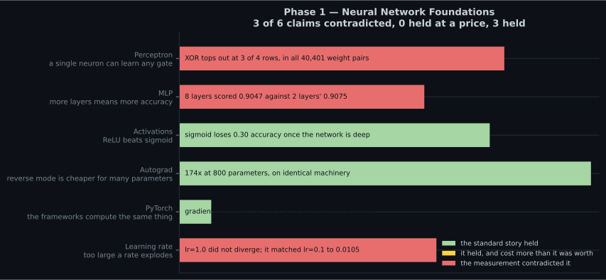
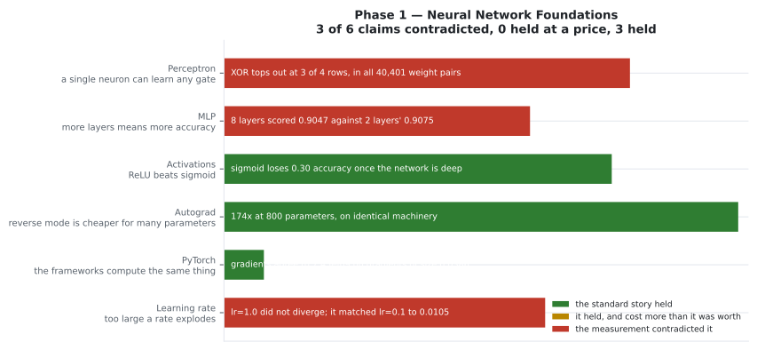
Six results that contradict the usual story
Section titled “Six results that contradict the usual story”The measurements in this phase are not all confirmations. Six worth knowing before you start, each with its evidence on the page it comes from:
- A learning rate 1,000× too small looks exactly like a broken model. At lr=0.0001 the network reached 0.1320 accuracy — barely above guessing — while its loss visibly moved. Sweep the rate before suspecting the architecture. (405.5)
- lr=1.0 did not diverge. The textbook picture says it should. On a shallow ReLU network with cross-entropy it matched lr=0.1 almost exactly, because the actual curvature was gentler than the theory’s worst case. (405.5)
- Plain SGD beat both momentum and Adam by three orders of magnitude on a clean two-parameter quadratic. Adaptive optimisers earn their keep on messy high-dimensional losses, not everywhere. (405.5)
- tanh beat ReLU at depth 8 (0.8782 against 0.8502) on the same data and seed. ReLU is the right default, not a law. (404)
- Logistic regression got 0.8618 on IMDB where the neural network got 0.8792. Most of the signal in a bag-of-words representation is linear. Without the baseline, 0.8792 sounds like a triumph. (406)
- A model with 0.7703 accuracy never predicted 13 of its 46 classes. Accuracy on imbalanced data measures the majority classes and almost nothing else. (407)
None of these are exotic edge cases. They are what happened when ordinary claims were checked on ordinary hardware.
Prerequisites
Section titled “Prerequisites”- The Machine Learning module, or comfort with train/test splits, loss functions and gradient descent.
- NumPy: array indexing,
shape,dtype, and basic broadcasting. - Python functions, classes and f-strings.
A quick self-test — if you can predict all four lines, you are ready:
import numpy as np

a = np.zeros((3, 4))
b = np.array([1.0, 2.0, 3.0, 4.0])
print((a + b).shape)                      # (3, 4) -- broadcasting
print(a.T.shape)                          # (4, 3)
print(np.dot(a, b.reshape(4, 1)).shape)   # (3, 1)
print(a.dtype)                            # float64
What you will need installed
Section titled “What you will need installed”pip install tensorflow numpy matplotlib scikit-learnEverything in this phase runs on a CPU. The slowest single measurement on any page
took 34 minutes — a deliberate batch-size-8 comparison, reported once and not
repeated — and the rest complete in seconds to a couple of minutes. No GPU, no
cloud account. Phase 1 is Keras and NumPy throughout, with one exception: page 405.9 installs torch to check, by measurement, how much of what you have learned is about neural networks rather than about TensorFlow.
By the end of this phase you can
Section titled “By the end of this phase you can”- Read and reason about tensor shapes, and predict when a broadcast will fail.
- Compute a layer’s parameter count by hand and check it against
model.count_params(). - Choose an output layer and loss for binary, multiclass and regression targets, and explain why each pairing exists.
- Derive one gradient-descent step by hand and reproduce an optimiser’s update exactly.
- Write reverse-mode autodiff from scratch, so
GradientTapestops being magic. - Build a model in any of the three Keras APIs and pick the right one for a given architecture.
- Establish a baseline before training anything, and recognise when a network is not beating it.
- Read training curves to find the epoch to stop at, and explain why validation loss and validation accuracy disagree about when that is.
- Report a result honestly: per-class recall on imbalanced data, K-fold spread on small data, residuals rather than averages.
Phase 1’s networks were shallow — two or three layers — because deeper ones do not train without help. Phase 2 covers what that help is: weight initialisation, normalisation layers, better optimisers, dropout, and the rest of the machinery that makes depth work at all.
-
Why does this phase insist on measuring a baseline before building a network?
A number with nothing to compare it against is not a measurement. This is the most transferable habit in the phase.
pch.quizShowAnswer
B — Because without it you cannot tell whether a result is good — logistic regression scored 0.8618 on IMDB where the network scored 0.8792, a gap that only means something once you know the baseline — A number with nothing to compare it against is not a measurement. This is the most transferable habit in the phase.
-
Which order should the ten pages be read in?
The worked examples at 406-408 assume the loss functions, output layers and training loop built on every earlier page.
pch.quizShowAnswer
B — In sidebar order: tensors, perceptron, MLP, activations, Keras, gradient descent, autograd, then the three worked examples, which reuse everything before them — The worked examples at 406-408 assume the loss functions, output layers and training loop built on every earlier page.
-
The phase reports that tanh beat ReLU at depth 8, and that plain SGD beat Adam on a quadratic. What is the intended lesson?
Both results are narrow and reproducible. ReLU and Adam remain the sensible starting points; the habit of checking is the part that transfers.
pch.quizShowAnswer
B — Defaults are defaults, not laws — they are usually right, and the only way to know whether they are right for your problem is to measure it — Both results are narrow and reproducible. ReLU and Adam remain the sensible starting points; the habit of checking is the part that transfers.
-
What hardware does Phase 1 require?
The heaviest single run took 34 minutes and was included deliberately to show what a bad batch size costs. Everything else is seconds to minutes.
pch.quizShowAnswer
B — A CPU — every measurement in the phase was produced on one, using only TensorFlow, NumPy, matplotlib and scikit-learn — The heaviest single run took 34 minutes and was included deliberately to show what a bad batch size costs. Everything else is seconds to minutes.
pch.coffeeTagline
pch.coffeeCtapch.feedbackHeading
pch.feedbackSubheading