Batch Normalization

Careful initialisation sets the activation variance to 1 at step zero. Nothing holds it there once the weights start moving. Batch normalisation gives up on hoping and simply recomputes the statistics at every layer, on every batch — which turns out to fix more than it was designed for, and to break in one specific way worth knowing about.

What you’ll learn

• The four-step BN forward pass, implemented by hand and matched to Keras within 1.61e−06.
• A 10-layer sigmoid network going from 0.1025 accuracy without BN to 0.9225 with it.
• Why BN behaves differently in fit and predict, measured: a moving mean of 27.52 against a true mean of 101.56 after three batches.
• What momentum costs you: 459 batches at the default 0.99 to get within 1%, and 4,603 at 0.999.
• BN’s real practical benefit: at lr = 1.0 it scored 0.9380 where the same network without BN collapsed to 0.3985.
• The failure case: at batch size 4 BN was worse than no BN (0.8680 against 0.8830).
• What BN adds to the parameter count, and why half of it is non-trainable.

What the layer does

For each feature, over the current mini-batch $B$:

$$\mu_B = \frac{1}{m}\sum_{i=1}^{m} x_i \qquad \sigma_B^2 = \frac{1}{m}\sum_{i=1}^{m}(x_i - \mu_B)^2$$ $$\hat{x}_i = \frac{x_i - \mu_B}{\sqrt{\sigma_B^2 + \epsilon}} \qquad y_i = \gamma \hat{x}_i + \beta$$

Normalise, then scale and shift by two learned parameters. The scale-and-shift is not decoration: without it the layer would force every activation distribution to be zero-mean and unit-variance, which is a constraint the network never asked for. With $\gamma$ and $\beta$ trainable, the network can undo the normalisation wherever that is what it needs — including recovering the identity exactly.

Implemented by hand on a batch with wildly different feature scales:

Column	Mean before	Std before	Mean after	Std after
0	−0.4582	0.8560	0.0000	0.9993
1	10.0685	3.4553	−0.0000	1.0000
2	−3.0483	0.1698	−0.0000	0.9831
3	101.5604	13.2305	0.0000	1.0000

Maximum difference against keras.layers.BatchNormalization(training=True): 1.61e−06. $\gamma$ initialises to 1 and $\beta$ to 0, so an untrained BN layer is exactly the normalisation.

The standard deviations after are 0.9993 and 0.9831 rather than 1.0000 because of the $\epsilon = 10^{-3}$ in the denominator — it matters most for column 2, whose variance was only 0.029, so the $\epsilon$ is a noticeable fraction of it.

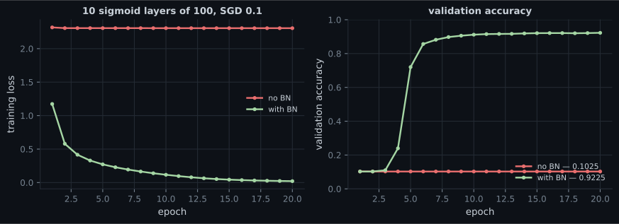
The case it was invented for

Ten sigmoid layers of 100 units, SGD at 0.1, twenty epochs, identical seeds:

figure 10 sigmoid layers of 100, SGD 0.1 matplotlib

Without BN this network never learns anything at all: its loss sits at 2.3056 and its accuracy at 0.1025 for twenty epochs, exactly the ln(10) = 2.3026 signature of a uniform prediction. With BN inserted before each activation, the same architecture and seed reaches 0.9225. Note that BN needed three epochs before anything happened — normalising does not remove the need to warm up.

	Final training loss	Final validation accuracy
no BN	2.3056	0.1025
with BN	0.0210	0.9225

This is not a marginal improvement; it is the difference between a network and a random-number generator. Ten stacked sigmoids give a gradient product bounded by $0.25^{10} \approx 9.5\times 10^{-7}$, as derived on the vanishing gradients page. BN resets the scale at every layer, so the product never gets the chance to collapse.

BN goes between the linear step and the activation

keras.layers.Dense(100, use_bias=False),      # BN's beta replaces the bias
keras.layers.BatchNormalization(),
keras.layers.Activation("relu"),

use_bias=False on the preceding Dense is not an optimisation detail: BN subtracts the batch mean, which removes any constant the bias added. The bias becomes a parameter with no effect on the output, and $\beta$ does that job instead.

diagram Diagram mermaid

  flowchart LR
  A["Dense
use_bias=False"] --> B["BatchNormalization"]
  B --> C["Activation"]
  C --> D["next layer"]
  E["training: batch mean and variance
+ update the moving averages"] -.-> B
  F["predict: the stored moving averages
nothing is recomputed"] -.-> B

Two modes, and the gap between them

BN is one of the few layers that computes something different during fit than during predict. In training it uses the current batch’s statistics. At inference there may be no batch — you might be scoring one row — so it uses a running average accumulated during training.

Measured on a fixed batch, calling the layer three times in training mode and then once in inference mode:

Call	Mean of column 3 in the output	moving_mean[3]
training 1	0.000000	10.156040
training 2	0.000000	19.296476
training 3	0.000000	27.522869
predict	10.667809	27.522869

The true mean of that column is 101.5604. In training mode the output is centred by construction — that is what the layer does. In inference mode it subtracts 27.52 instead of 101.56, so the output is not centred at all, and will not be until the moving average has caught up.

This is the source of the classic “my model scores well during training and badly at predict time” bug. Nothing is wrong with the model; the moving statistics have not converged.

The momentum hyperparameter

$$\text{moving} \leftarrow \text{momentum} \cdot \text{moving} + (1 - \text{momentum}) \cdot \text{batch}$$

Starting from zero, how long until the estimate reaches within 1% of a true value of 100?

momentum	After 10 batches	After 50	After 200	Batches to reach 99%
0.9	65.1322	99.4846	100.0000	44
0.99 (Keras default)	9.5618	39.4994	86.6020	459
0.999	0.9955	4.8794	18.1351	4,603

At the default 0.99 you need roughly 459 optimisation steps before the inference path is trustworthy. On 8,000 rows at batch 128 that is 63 steps per epoch — so seven epochs before the moving statistics are within 1%. Validate after one epoch and the result is meaningless.

Lower the momentum for short runs or small datasets; raise it for very long runs where you want a smoother estimate.

sketch Watch the moving average catch up p5.js Pause Restart

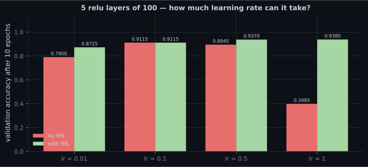
The exact recursion Keras uses, drawn for a true value of 100. Drag the momentum slider and see how many batches the inference path needs before it can be trusted.

What BN actually buys on a normal network

Five ReLU layers of 100 — a network that trains perfectly well without help — at four learning rates:

figure 5 relu layers of 100 — how much learning rate can it take? matplotlib

At the well-tuned rate of 0.1 the two are exactly equal at 0.9115: BN bought nothing. Its value shows up at the edges — 0.8725 against 0.7900 when the rate is too small, and 0.9380 against 0.3985 when it is ten times too large. BN widens the range of learning rates that work rather than improving the best one.

Learning rate	no BN	with BN
0.01	0.7900	0.8725
0.1	0.9115	0.9115
0.5	0.8945	0.9370
1.0	0.3985	0.9380

At the well-chosen rate the two are identical to four decimal places. That is the honest headline: BN did not make this network better, it made it harder to break. With BN the worst of four learning rates scored 0.8725; without it, 0.3985. That is why BN lets you use larger rates and shorter schedules — not because it raises the ceiling.

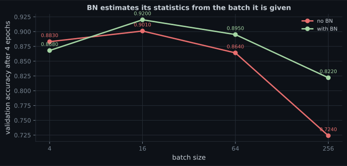
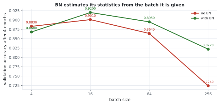
Where BN fails: small batches

The statistics come from the batch. A batch of 4 gives a 4-sample estimate of a mean and variance, which is mostly noise.

figure BN estimates its statistics from the batch it is given matplotlib

At batch 4 BN scored 0.8680 against 0.8830 without it — the only point where BN loses. From batch 16 upward BN is ahead, by 0.019, 0.031 and 0.098. Small-batch training is exactly the regime where LayerNormalization or GroupNormalization are preferred, because neither depends on the batch dimension.

Batch size	no BN	with BN
4	0.8830	0.8680
16	0.9010	0.9200
64	0.8640	0.8950
256	0.7240	0.8220

Two things fall out of that table. BN’s advantage grows with batch size, because its estimates get better. And it goes negative at batch 4, because a four-sample variance is worse than no normalisation at all. If your batch has to be small — large images, long sequences, memory limits — use LayerNormalization, which normalises across features within each sample and never touches the batch axis.

The parameter cost

	Total	Trainable	Non-trainable
3 layers, no BN	99,710	99,710	0
3 layers, with BN	100,610	100,010	600

Each BN layer stores four values per feature: $\gamma$ and $\beta$ are trained, moving_mean and moving_variance are not. For three layers of 100 features that is 600 trainable and 600 non-trainable values, while use_bias=False removes 300 biases — so the trainable count rises by 300 and the total by 900.

Those non-trainable values are part of the model’s state. They are saved with the weights and they must be, or your restored model will normalise with the wrong statistics. model.save handles this; hand-rolled weight copying often does not.

sketch The measured table, ranked p5.js Pause Restart

Click a column to rank every row by it. The bars are that column's values and the highest and lowest are computed from the numbers, not written in.

Pitfalls

• Validating before the moving statistics converge. At the default momentum=0.99 that takes 459 batches. Early validation scores can look catastrophic for no real reason.
• Keeping use_bias=True before a BN layer. The bias has no effect — BN subtracts the mean — so it is a wasted parameter.
• Using BN with a batch size below about 16. Measured, BN lost to no-BN at batch 4. Use LayerNormalization there.
• Assuming BN improves the best achievable score. At the well-tuned learning rate here, BN and no-BN tied at 0.9115 exactly.
• Forgetting the non-trainable weights when copying weights by hand. moving_mean and moving_variance are model state.
• Stacking BN and dropout in the same block carelessly. Dropout changes the activation variance that BN just standardised; if you use both, dropout goes after BN, and expect to retune both.
• Fine-tuning with BN layers left trainable on a tiny dataset. The moving statistics get overwritten with estimates from a handful of batches. Freeze them or lower the momentum deliberately.

Recap

• BN normalises each feature over the mini-batch, then applies a learned scale $\gamma$ and shift $\beta$ — verified against Keras to 1.61e−06.
• On ten stacked sigmoid layers it took validation accuracy from 0.1025 (a uniform prediction) to 0.9225.
• Training mode uses batch statistics; inference mode uses a moving average that lags — 27.52 against a true 101.56 after three batches.
• momentum=0.99 needs 459 batches to get within 1% of the truth; 0.999 needs 4,603.
• On a network that already trains, BN’s benefit is tolerance rather than accuracy: identical at lr=0.1, but 0.9380 against 0.3985 at lr=1.0.
• BN loses at batch 4 (0.8680 against 0.8830) and its advantage grows with batch size. Small batches want LayerNormalization.
• Each BN layer adds four values per feature; two are trainable, two are model state that must be saved.

Next

BN keeps the signal well-scaled. It does not stop a model from memorising its training set — that needs a different kind of pressure: Regularization & Dropout.

pch.quizTag pch.quizDefaultTitle

1. Your model reports 0.95 training accuracy but 0.30 when you call predict on the same data, and you are using BatchNormalization. What is the most likely cause?

   A The model is overfitting B The moving statistics have not converged: at momentum=0.99 they need about 459 batches, and until then predict normalises with badly wrong mean and variance estimates C predict applies dropout as well D The data needs rescaling before predict
   pch.quizShowAnswer

   B — The moving statistics have not converged: at momentum=0.99 they need about 459 batches, and until then predict normalises with badly wrong mean and variance estimates — Measured: after three batches the moving mean was 27.52 against a true 101.56. Train longer, lower the momentum, or both.

2. Why is use_bias=False recommended on a Dense layer immediately followed by BatchNormalization?

   A It makes the layer faster to compute B BN subtracts the batch mean, which cancels any constant the bias added — so the bias cannot affect the output, and BN's own beta parameter plays that role instead C Biases interfere with the gamma parameter D It is required; Keras raises an error otherwise
   pch.quizShowAnswer

   B — BN subtracts the batch mean, which cancels any constant the bias added — so the bias cannot affect the output, and BN's own beta parameter plays that role instead — The bias becomes a parameter with literally no effect. Removing it costs nothing and saves one value per unit.

3. At learning rate 0.1 the network scored 0.9115 both with and without BN, but at 1.0 the scores were 0.9380 and 0.3985. What does that pattern mean?

   A BN only helps at high learning rates and should not be used otherwise B BN's benefit is widening the range of learning rates that work, not raising the best achievable score — it makes training robust rather than better C The lr=0.1 measurement must be wrong D BN removes the need to tune the learning rate at all
   pch.quizShowAnswer

   B — BN's benefit is widening the range of learning rates that work, not raising the best achievable score — it makes training robust rather than better — That robustness is what lets practitioners use larger rates and shorter schedules, which is a real speed benefit — just not an accuracy one.

4. At batch size 4, BN scored 0.8680 against 0.8830 without it. Why?

   A Small batches make the gradients too noisy for any layer to work B BN estimates the mean and variance from the batch it is given, and a four-sample estimate is mostly noise — so the normalisation injects error rather than removing it C BN requires at least 32 samples by construction D The learning rate was wrong for that batch size
   pch.quizShowAnswer

   B — BN estimates the mean and variance from the batch it is given, and a four-sample estimate is mostly noise — so the normalisation injects error rather than removing it — This is the regime where LayerNormalization is preferred: it normalises across features within each sample, so the batch size is irrelevant to it.

5. A BN layer over 100 features adds how many values, and how many of them are trained?

   A 100 values, all trained B 400 values: gamma and beta (200) are trained, while moving_mean and moving_variance (200) are non-trainable model state that must still be saved with the weights C 200 values, all trained D None — BN has no parameters
   pch.quizShowAnswer

   B — 400 values: gamma and beta (200) are trained, while moving_mean and moving_variance (200) are non-trainable model state that must still be saved with the weights — Forgetting the non-trainable half is a common bug when copying weights by hand: the restored model then normalises with the wrong statistics.

🧪 Try It Yourself

pch.exerciseTag pch.exerciseTitle

pch.exerciseTag pch.exerciseTitle

pch.exerciseTag pch.exerciseTitle

pch.exerciseTag pch.exerciseTitle

pch.exerciseTag pch.exerciseTitle

pch.exerciseTag pch.exerciseTitle