
Capstone 1 - Fraud Screening End to End
The decision
Section titled “The decision”A payments team screens transactions. Flagged ones go to a human reviewer; unflagged ones settle.
| Who acts | Six analysts, each reviewing about 50 alerts a shift |
| Cost of a review | EUR 5 |
| Cost of a missed fraud | EUR 500 on average, or the transaction amount when known |
| Base rate | 0.43% of transactions |
The deliverable is not a model. It is a threshold, an alert volume, and an expected loss per transaction — three numbers the business can act on, plus the evidence that the model reads what a fraud analyst would expect it to read.
This capstone composes five earlier pages: the metric choice, the cost-derived threshold, the importance audit, the segment check and the schema contract.
Step 1 — split three ways, and pick the metric first
Section titled “Step 1 — split three ways, and pick the metric first”# 50% to fit, 20% to choose operating points, 30% to report once
X_fit, X_rest, y_fit, y_rest, a_fit, a_rest = train_test_split(
X, y, amount, test_size=0.5, random_state=0, stratify=y)
X_val, X_te, y_val, y_te, a_val, a_te = train_test_split(
X_rest, y_rest, a_rest, test_size=0.6, random_state=0, stratify=y_rest)
# fit 10,000 / 44 frauds val 4,000 / 17 test 6,000 / 26| Metric | Value | Why it is here |
|---|---|---|
| accuracy | not reported | 0.9958 here, and 0.9957 for a model that does nothing |
| average precision | 0.4387 | chance is the base rate, 0.0043 — a 101× lift |
| Brier score | 0.003160 | the threshold rule needs calibrated probabilities |
| ROC-AUC | secondary | flattering under imbalance |
Average precision is the headline because the review workload scales with alerts, and Brier is on the list because the next step consumes probabilities rather than a ranking.
Step 2 — turn the costs into a policy
Section titled “Step 2 — turn the costs into a policy”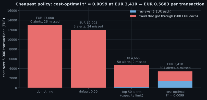
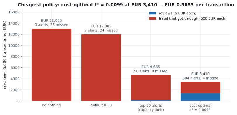
| Policy | Alerts | False alerts | Missed | Precision | Recall | Total cost |
|---|---|---|---|---|---|---|
| do nothing | 0 | 0 | 26 | — | 0.0000 | EUR 13,000 |
| default 0.50 | 3 | 1 | 24 | 0.6667 | 0.0769 | EUR 12,005 |
| top 50 by score (capacity) | 50 | 33 | 9 | 0.3400 | 0.6538 | EUR 4,665 |
| cost-optimal | 304 | 282 | 4 | 0.0724 | 0.8462 | EUR 3,410 |
| per-row , loss = the amount | 80 | 64 | 10 | 0.2000 | 0.6154 | EUR 853 † |
† The last row is priced against the transaction amount rather than a flat EUR 500, so its total is not comparable with the rows above it. Within that costing it is the cheapest policy available.
Three numbers to carry into the meeting:
- Expected loss per transaction: EUR 0.5683 at , against EUR 2.1667 doing nothing. That is the business case, and it is a per-unit number so it scales.
- 304 alerts per 6,000 transactions — 5.1% of volume. At six analysts × 50 alerts that is a hard constraint, and the model does not get to ignore it.
- The capacity policy costs EUR 1,255 more than the unconstrained optimum. That difference is the value of hiring the seventh analyst, expressed in the same units as their salary.
See it move
Section titled “See it move”The four policies in that table are four points on one curve. The sketch is that curve, measured on the same 6,000 test transactions at 43 thresholds — drag the threshold and read the alert count, the misses and the bill. The analyst-capacity line at 50 alerts is drawn where operations actually sits.
One honest wrinkle the curve exposes: on this particular test set the cheapest threshold measured is 0.00346 at EUR 2,675, not at EUR 3,410. That is not evidence that the formula is wrong — with 26 frauds, the realised cost of any threshold has a standard error of hundreds of euros, and the empirical argmin is itself a selected number with exactly the winner’s curse built in. minimises expected cost from the cost ratio alone and needs no tuning; the empirical minimum minimises this sample and would move on the next one. Ship the formula, and note the flat bottom: anything from roughly 0.003 to 0.04 costs under EUR 4,000, so the decision is robust even though the argmin is not.
Step 3 — audit what the model reads
Section titled “Step 3 — audit what the model reads”Permutation importance on the test set, scored by average precision, 20 repeats:
| Feature | Δ average precision |
|---|---|
geo_mismatch | +0.3887 ± 0.0138 |
velocity | +0.3374 ± 0.0242 |
amount_z | +0.2557 ± 0.0423 |
device_age | +0.2500 ± 0.0346 |
hour_z | +0.1499 ± 0.0542 |
noise | −0.0011 ± 0.0052 |
Two checks pass here. The five features a fraud analyst would name are the five that matter, in a
plausible order. And the deliberately uninformative column scores −0.0011 ± 0.0052 — indistinguishable
from zero, which is what a column of noise should score. Had noise ranked third, the correct response
would be to stop and find out why, exactly as on
the shortcut page.
Step 4 — check the segments before shipping
Section titled “Step 4 — check the segments before shipping”The model never sees the channel a transaction arrived through. Slice the results by it anyway:
| Channel | n | Frauds | Alerts | Precision | Recall |
|---|---|---|---|---|---|
| web | 3,268 | 13 | 172 | 0.0698 | 0.9231 |
| app | 2,128 | 9 | 103 | 0.0680 | 0.7778 |
| phone | 604 | 4 | 29 | 0.1034 | 0.7500 |
Recall ranges from 0.7500 to 0.9231 across channels. Before treating that as a finding, note the denominators: 4 frauds in the phone segment. One fraud either way moves that recall by 0.25, so the honest statement is “no measurable difference between channels, and the phone segment is too small to tell” — the same discipline as any fairness slice. What you can commit to is monitoring it monthly, when the counts accumulate.
Step 5 — the engineering that makes it a system
Section titled “Step 5 — the engineering that makes it a system”CONFIG = {"c_fp": 5.0, "c_fn": 500.0, "model_version": "fraud-1.2.0"}
def screen(batch, artefact, config):
"""One batch: validate, score, threshold, and log everything an audit needs."""
problems = validate(batch, artefact["schema"])
hard = [p for p in problems if "column" in p or "null rate" in p]
if hard:
raise ValueError(f"unusable batch: {hard}") # do not predict
proba = artefact["model"].predict_proba(batch)[:, 1]
threshold = config["c_fp"] / (config["c_fp"] + config["c_fn"])
flagged = proba >= threshold
return {
"model_version": config["model_version"],
"schema_id": artefact["schema_id"],
"threshold": threshold,
"rows": len(batch),
"alerts": int(flagged.sum()),
"alert_rate": round(float(flagged.mean()), 4),
"mean_score": round(float(proba.mean()), 6),
"warnings": problems, # statistics, not structure
"scores": proba, # logged per row
}Four things this earns:
- Hard-fail on structure, warn on statistics — the policy from the validation page.
alert_rateis the operational canary. It is available immediately, needs no labels, and a jump from 5.1% to 12% means something changed today, whatever the labels eventually say.mean_scorecatches recalibration. The model’s mean predicted probability should track the base rate (0.0043 here). A drift in it invalidates the threshold, because assumes calibration.- The threshold is derived from config, never hard-coded. When finance revises the fraud cost, one number changes and nothing retrains.
The test suite, from Testing ML Code:
a metric floor (average precision ≥ 0.30 on the fixed split), memorisation of 24 rows, a directional
expectation on velocity, a structural assertion that the scaler is inside the Pipeline, and a schema
round-trip.
The system those pieces add up to, with the two feedback paths that make it survive contact with production:
  flowchart TD
  B["incoming batch of transactions"] --> V{{"validate against
the schema artefact"}}
  V -->|"structural problem:
missing column, null rate"| STOP["raise. do not predict.
a wrong answer is worse
than no answer"]
  V -->|"statistical warning:
range, mean shift"| LOGW["log the warning
and continue"]
  V -->|"clean"| SCORE
  LOGW --> SCORE["model.predict_proba
fraud-1.2.0"]
  CFG[("config:
c_fp = 5, c_fn = 500")] -->|"t* = c_fp / (c_fp + c_fn)"| THR{{"threshold at 0.0099"}}
  SCORE --> THR
  THR -->|"score >= t*"| Q["alert queue,
ranked by score"]
  THR -->|"score < t*"| PASS["let through"]
  Q --> CAP{{"analyst capacity:
50 reviews per shift"}}
  CAP -->|"within capacity"| REV["human review"]
  CAP -->|"queue longer than capacity"| SPILL["review top-ranked only.
the overflow is an
accepted, measured loss"]
  SCORE --> MON["log alert_rate and mean_score
-- no labels needed"]
  MON -->|"alert_rate jumps 5.1% -> 12%,
or mean_score leaves 0.0043"| INV["investigate today:
upstream change, or
the threshold is stale"]
  REV --> LAB["confirmed labels,
weeks later"]
  SPILL --> LAB
  LAB --> RETRAIN["retrain and re-audit;
recompute t* if finance
revises the costs"]
  RETRAIN -.-> SCORE
  INV -.-> CFG
Note what is not in the model: the capacity constraint, the cost ratio and the review workflow all
live in configuration and operations. That separation is what lets finance change c_fn on a Tuesday
without a retraining run, and it is the difference between a model and a system.
What this project does not solve
Section titled “What this project does not solve”- The 26 test frauds. Every number here has a wide confidence interval; the bootstrap on this data spanned 0.37 of average precision. Treat model comparisons as inconclusive until far more positives accumulate.
- Label delay. Chargebacks arrive weeks later, so today’s recall is unknowable today. The alert rate and score distribution are the only same-day signals.
- Adversarial drift. Fraud patterns react to the screening policy. Nothing on this page models an adversary who learns your threshold.
- The review process. A 93%-false-alert queue has a human cost — fatigue, inconsistency — that the EUR 5 does not capture.
- 6,000 test transactions, 26 frauds (0.43%); average precision 0.4387 against a 0.0043 chance line.
- The default threshold cost EUR 12,005 against EUR 13,000 for doing nothing.
- cost EUR 3,410: 304 alerts, 4 missed, precision 0.0724, recall 0.8462.
- Expected loss per transaction: EUR 0.5683 against EUR 2.1667.
- A 50-alert capacity limit cost EUR 4,665 — EUR 1,255 more than the unconstrained optimum.
- The audit passed: the five plausible features led, and
noisescored −0.0011 ± 0.0052. - Channel recall ranged 0.7500–0.9231 on 4–13 frauds per segment: no measurable difference.
-
Your fraud screener has precision 0.0724 at the cost-optimal threshold. How do you present it?
93% false alerts is the correct policy when a missed fraud costs 100 reviews, and it is also the number most likely to get the project cancelled. Per-transaction expected loss is the unit the business already thinks in.
pch.quizShowAnswer
B — As money: EUR 1,410 of reviews avoids EUR 11,000 of losses, and expected loss per transaction falls from 2.1667 to 0.5683 — 93% false alerts is the correct policy when a missed fraud costs 100 reviews, and it is also the number most likely to get the project cancelled. Per-transaction expected loss is the unit the business already thinks in.
-
Analysts can review 50 alerts a shift; the cost-optimal policy produces 304. What is the useful thing to compute?
You will ship the capacity-limited policy either way. Quantifying the constraint in euros turns 'the model is noisy' into 'a seventh analyst pays for themselves', which is a decision someone can make.
pch.quizShowAnswer
B — Both: the top-50 policy costs EUR 4,665 against EUR 3,410 unconstrained, so the EUR 1,255 gap is the value of additional review capacity — You will ship the capacity-limited policy either way. Quantifying the constraint in euros turns 'the model is noisy' into 'a seventh analyst pays for themselves', which is a decision someone can make.
-
The 'noise' feature scores -0.0011 ± 0.0052 in the permutation audit. What does that establish?
The point of including a known-useless column is to calibrate your reading of the others. Had it ranked third, the deployment would stop until someone explained why.
pch.quizShowAnswer
B — That the audit is working: a column with no information scores indistinguishably from zero, which is what makes the five leading features credible — The point of including a known-useless column is to calibrate your reading of the others. Had it ranked third, the deployment would stop until someone explained why.
-
Recall by channel is 0.9231 (web), 0.7778 (app), 0.7500 (phone). Is the model worse for phone customers?
Segment metrics need denominators printed next to them. With 4, 9 and 13 positives these three numbers are compatible with identical underlying performance, and acting on them would be acting on noise.
pch.quizShowAnswer
B — Unknown: the phone segment contains 4 frauds, so one either way moves recall by 0.25 — report 'no measurable difference' and monitor monthly — Segment metrics need denominators printed next to them. With 4, 9 and 13 positives these three numbers are compatible with identical underlying performance, and acting on them would be acting on noise.
-
Which same-day signal tells you the screener has broken, before any chargeback arrives?
Labels arrive weeks late, so every label-based metric is stale by construction. A jump in alert rate from 5.1% to 12%, or a mean score that stops tracking the base rate, is actionable today — and a drifting mean score also invalidates the threshold, which assumes calibration.
pch.quizShowAnswer
B — The alert rate and the mean predicted score — both available immediately and both invalidated by the changes that matter — Labels arrive weeks late, so every label-based metric is stale by construction. A jump in alert rate from 5.1% to 12%, or a mean score that stops tracking the base rate, is actionable today — and a drifting mean score also invalidates the threshold, which assumes calibration.
🧪 Try It Yourself
Section titled “🧪 Try It Yourself”Exercise 1 – Build the screening dataset and split it three ways
Section titled “Exercise 1 – Build the screening dataset and split it three ways”Exercise 2 – Report the right metric
Section titled “Exercise 2 – Report the right metric”Exercise 3 – Price four policies
Section titled “Exercise 3 – Price four policies”Exercise 4 – Audit what the model reads
Section titled “Exercise 4 – Audit what the model reads”Exercise 5 – Slice by a segment the model never saw
Section titled “Exercise 5 – Slice by a segment the model never saw”Capstone 2 - Churn with Point-in-Time Features — the same decision structure on an event log, where the hard part is not the model but making sure the features could have existed when the prediction was made.
pch.coffeeTagline
pch.coffeeCtapch.feedbackHeading
pch.feedbackSubheading