Matrix Approximation

The SVD gave you an exact factorisation. This page throws part of it away on purpose.

The result is remarkable and it is easy to under-appreciate: if you keep only the largest $k$ singular values, the matrix you get back is not merely a good rank-$k$ approximation — it is the best one that exists, and its error is exactly $\sigma_{k+1}$. Not bounded by, not approximately: equal to. You know the error before you compute the approximation.

What you’ll learn

• Equations 4.90 and 4.91: any rank-$r$ matrix is a sum of $r$ rank-1 outer products, weighted by the singular values.
• Equation 4.92: truncating that sum at $k$ gives the rank-$k$ approximation $\hat{\mathbf{A}}(k)$.
• Definition 4.23 and Theorem 4.24: the spectral norm, and the fact that it equals $\sigma_1$.
• Theorem 4.25, Eckart-Young: the truncation is optimal, and $\lVert\mathbf{A} - \hat{\mathbf{A}}(k)\rVert_2 = \sigma_{k+1}$.
• The sketch of why no rank-$k$ matrix can do better, via the rank-nullity theorem.
• Example 4.15: reading two themes out of a movie-ratings matrix — and a transcription error in the book’s Equation 4.101b, diagnosed exactly.
• The storage arithmetic: when a factorisation actually saves anything, and when it does not.

Intuition: a matrix as a stack of transparencies

An outer product $\mathbf{u}\mathbf{v}^\top$ is the simplest nonzero matrix there is. Every row is a multiple of $\mathbf{v}^\top$ and every column is a multiple of $\mathbf{u}$, so it has rank 1 and it looks like a grid — one column pattern times one row pattern, and nothing else. The book makes exactly this point about Figure 4.11: the grid-like structure of each rank-1 matrix is imposed by the outer-product of the left and right-singular vectors.

The SVD says every matrix is a weighted stack of these transparencies, and it orders them by weight. The first carries the most; the last carries the least. Approximating is then simply not laying down the faint ones.

What makes it a theorem rather than a heuristic is that this particular stack is the right one. You could decompose a matrix into rank-1 pieces in infinitely many ways; only the SVD’s ordering has the property that the first $k$ pieces are the best $k$ pieces.

diagram Diagram mermaid

  flowchart TD
  A["A, rank r"] --> SUM["A = Σᵢ σᵢ uᵢ vᵢᵀ
Eq 4.91: a weighted sum
of r rank-1 matrices"]
  SUM --> WHY["why: Σ is diagonal, so it pairs
only matching uᵢ with vᵢ;
terms i > r vanish because σᵢ = 0"]
  SUM --> TRUNC["stop at k < r
Â(k) = Σᵢ₌₁ᵏ σᵢ uᵢ vᵢᵀ
Eq 4.92, rank exactly k"]
  TRUNC --> DIFF["A − Â(k) = Σᵢ₌ₖ₊₁ʳ σᵢ uᵢ vᵢᵀ
Eq 4.96 — the leftovers"]
  NORM["spectral norm ‖A‖₂ = maxₓ ‖Ax‖₂/‖x‖₂
Def 4.23"] --> T424["Thm 4.24: ‖A‖₂ = σ₁"]
  DIFF --> T424
  T424 --> EY["Thm 4.25 Eckart-Young
‖A − Â(k)‖₂ = σₖ₊₁
and no rank-k B does better"]
  EY --> USE["lossy compression, denoising,
regularising ill-posed problems,
and PCA in Chapter 10"]

The math

Every matrix is a sum of rank-1 pieces

Define the outer-product matrices

$$\mathbf{A}_i := \mathbf{u}_i\mathbf{v}_i^\top \tag{4.90}$$

Then a matrix $\mathbf{A} \in \mathbb{R}^{m\times n}$ of rank $r$ satisfies

$$\mathbf{A} = \sum_{i=1}^{r} \sigma_i\mathbf{u}_i\mathbf{v}_i^\top = \sum_{i=1}^{r} \sigma_i\mathbf{A}_i \tag{4.91}$$

The book’s own reason is worth quoting because it is the whole argument: the diagonal structure of the singular value matrix $\boldsymbol{\Sigma}$ multiplies only matching left- and right-singular vectors $\mathbf{u}_i\mathbf{v}_i^\top$ and scales them by the corresponding singular value $\sigma_i$. All terms $\Sigma_{ij}\mathbf{u}_i\mathbf{v}_j^\top$ vanish for $i \neq j$ because $\boldsymbol{\Sigma}$ is a diagonal matrix. Any terms $i > r$ vanish because the corresponding singular values are $0$.

So Equation 4.91 is not a new fact. It is $\mathbf{U}\boldsymbol{\Sigma}\mathbf{V}^\top$ written out term by term.

Truncating

Equation 4.92 — rank-k approximation

If the sum runs only up to an intermediate value $k < r$, we obtain the rank-$k$ approximation

$$\hat{\mathbf{A}}(k) := \sum_{i=1}^{k}\sigma_i\mathbf{u}_i\mathbf{v}_i^\top = \sum_{i=1}^{k}\sigma_i\mathbf{A}_i$$

with $\mathrm{rk}(\hat{\mathbf{A}}(k)) = k$.

The rank is exactly $k$, not at most $k$, because the $\mathbf{u}_i$ are orthonormal and the $\sigma_i$ for $i \leq k \leq r$ are nonzero.

Measuring the error

To say how good an approximation is you need a norm on matrices. §3.1 gave norms on vectors; the analogue here is:

Definition 4.23 — Spectral Norm

For $\mathbf{x} \in \mathbb{R}^n\setminus\{\mathbf{0}\}$, the spectral norm of a matrix $\mathbf{A} \in \mathbb{R}^{m\times n}$ is

$$\lVert\mathbf{A}\rVert_2 := \max_{\mathbf{x}} \frac{\lVert\mathbf{A}\mathbf{x}\rVert_2}{\lVert\mathbf{x}\rVert_2} \tag{4.93}$$

Read it as: how long can any vector at most become when multiplied by $\mathbf{A}$? The subscript $2$ matches the Euclidean norm on vectors on the right-hand side.

Theorem 4.24

The spectral norm of $\mathbf{A}$ is its largest singular value $\sigma_1$.

The book leaves the proof as an exercise — it is Exercise 4.11, and the next page works it. The intuition is immediate from the geometry of §4.5: $\mathbf{V}^\top$ and $\mathbf{U}$ are rotations and change no length, so all the stretching is $\boldsymbol{\Sigma}$, and the most a unit vector can be stretched by a diagonal matrix is its largest entry.

The theorem

Theorem 4.25 — Eckart-Young Theorem (Eckart and Young, 1936)

Consider a matrix $\mathbf{A} \in \mathbb{R}^{m\times n}$ of rank $r$ and let $\mathbf{B} \in \mathbb{R}^{m\times n}$ be a matrix of rank $k$. For any $k \leq r$ with $\hat{\mathbf{A}}(k) = \sum_{i=1}^k \sigma_i\mathbf{u}_i\mathbf{v}_i^\top$ it holds that

$$\hat{\mathbf{A}}(k) = \operatorname*{argmin}_{\mathrm{rk}(\mathbf{B})=k}\lVert\mathbf{A}-\mathbf{B}\rVert_2 \tag{4.94}$$$$\bigl\lVert\mathbf{A}-\hat{\mathbf{A}}(k)\bigr\rVert_2 = \sigma_{k+1} \tag{4.95}$$

Two separate claims. Equation 4.94 is optimality: nothing of rank $k$ is closer. Equation 4.95 is exactness: the error is not bounded by $\sigma_{k+1}$, it equals it.

The second claim is nearly free. The difference is just the discarded tail,

$$\mathbf{A} - \hat{\mathbf{A}}(k) = \sum_{i=k+1}^{r}\sigma_i\mathbf{u}_i\mathbf{v}_i^\top \tag{4.96}$$

which is itself a matrix in SVD form whose largest singular value is $\sigma_{k+1}$ — so Theorem 4.24 gives Equation 4.95 immediately.

Why nothing of rank k does better

The book’s argument is a proof by contradiction and it is short enough to follow completely. Suppose some $\mathbf{B}$ with $\mathrm{rk}(\mathbf{B}) \leq k$ satisfied

$$\lVert\mathbf{A}-\mathbf{B}\rVert_2 < \bigl\lVert\mathbf{A}-\hat{\mathbf{A}}(k)\bigr\rVert_2 = \sigma_{k+1} \tag{4.97}$$

Then $\mathbf{B}$ has a null space $Z \subseteq \mathbb{R}^n$ of dimension at least $n-k$, and for $\mathbf{x} \in Z$ we have $\mathbf{B}\mathbf{x} = \mathbf{0}$, hence

$$\lVert\mathbf{A}\mathbf{x}\rVert_2 = \lVert(\mathbf{A}-\mathbf{B})\mathbf{x}\rVert_2 \tag{4.98}$$

and by the matrix version of Cauchy-Schwarz,

$$\lVert\mathbf{A}\mathbf{x}\rVert_2 \leq \lVert\mathbf{A}-\mathbf{B}\rVert_2\lVert\mathbf{x}\rVert_2 < \sigma_{k+1}\lVert\mathbf{x}\rVert_2 \tag{4.99}$$

But there is a $(k+1)$-dimensional subspace — spanned by $\mathbf{v}_1,\dots,\mathbf{v}_{k+1}$ — on which $\lVert\mathbf{A}\mathbf{x}\rVert_2 \geq \sigma_{k+1}\lVert\mathbf{x}\rVert_2$. Adding the dimensions of those two subspaces gives $(n-k) + (k+1) = n+1 > n$, so they must share a nonzero vector, which cannot satisfy both inequalities. That contradicts the rank-nullity theorem (Theorem 2.24). Hence no such $\mathbf{B}$ exists.

Notice what carried the argument: counting dimensions. Chapter 2’s rank-nullity theorem, which looked like bookkeeping at the time, is what makes the SVD optimal.

From the book

Section 4.6. Equation 4.90 defines the rank-1 outer products $\mathbf{A}_i$ and Equation 4.91 writes any rank-$r$ matrix as their weighted sum, with the book’s own explanation of why the off-diagonal terms vanish. Equation 4.92 defines the rank-$k$ approximation. Figures 4.11 and 4.12 show a $1432\times1910$ Stonehenge photograph, its first five rank-1 pieces with $\sigma_1 \approx 228\,052$ down to $\sigma_5 \approx 15\,436$, and the reconstructions, with the storage arithmetic $5\cdot(1432+1910+1) = 16\,715$ numbers against $1432\cdot1910 = 2\,735\,120$ — just above $0.6\%$. Definition 4.23 (Equation 4.93) gives the spectral norm and Theorem 4.24 identifies it with $\sigma_1$, leaving the proof as an exercise. Theorem 4.25 (Equations 4.94 and 4.95) is Eckart-Young, followed by the contradiction argument of Equations 4.96 to 4.99 resting on the rank-nullity theorem 2.24. Example 4.15 continues the movie-ratings example of §4.5.3 with Equations 4.100 to 4.103.

Worked example by hand

Example 4.15 — two themes in a ratings table

The matrix from Example 4.14, four movies by three viewers:

$$\mathbf{A} = \begin{bmatrix}5 & 4 & 1\\ 5 & 5 & 0\\ 0 & 0 & 5\\ 1 & 0 & 4\end{bmatrix} \tag{4.103}$$

with $\sigma = 9.643811,\ 6.363891,\ 0.705552$. The first rank-1 piece is

$$\mathbf{A}_1 = \mathbf{u}_1\mathbf{v}_1^\top = \begin{bmatrix}-0.6710\\ -0.7197\\ -0.0939\\ -0.1515\end{bmatrix} \begin{bmatrix}-0.7367 & -0.6515 & -0.1811\end{bmatrix} = \begin{bmatrix}0.4943 & 0.4372 & 0.1215\\ 0.5302 & 0.4689 & 0.1303\\ 0.0692 & 0.0612 & 0.0170\\ 0.1116 & 0.0987 & 0.0274\end{bmatrix} \tag{4.100}$$

Reproduced from the SVD to $6.7\times10^{-5}$, which is the rounding of the book’s four printed decimals. The book’s reading: Ali and Beatrix like science fiction — Star Wars and Blade Runner, entries above $0.4$ — but this piece fails to capture Chandra’s ratings, which is unsurprising, since Chandra’s taste is not in the first singular direction.

The second piece captures the other theme, French art house. Combining them,

$$\hat{\mathbf{A}}(2) = \sigma_1\mathbf{A}_1 + \sigma_2\mathbf{A}_2 = \begin{bmatrix}4.7801 & 4.2419 & 1.0244\\ 5.2252 & 4.7522 & -0.0250\\ 0.2493 & -0.2743 & 4.9724\\ 0.7495 & 0.2756 & 4.0278\end{bmatrix} \tag{4.102}$$

which reproduces Equation 4.102 to all four printed decimals. Compare against $\mathbf{A}$: every entry is within about $0.28$. The conclusion the book draws is that $\mathbf{A}_3$ can be ignored — there is no evidence of a third movie-theme category, and the whole space of themes is two-dimensional.

And Eckart-Young says exactly how good that is, before you look: $\lVert\mathbf{A}-\hat{\mathbf{A}}(2)\rVert_2 = \sigma_3 = 0.705552$. Measured on the book’s own printed $\hat{\mathbf{A}}(2)$: $0.705580$, the difference being the four-decimal rounding.

The book’s Equation 4.101b uses the wrong vector — diagnosed

Work through Equation 4.101 and it does not come out. The printed $\mathbf{v}_2^\top = [0.0852,\ 0.1762,\ -0.9807]$ is the second row of $\mathbf{V}^\top$, which is correct — but the matrix printed as $\mathbf{A}_2$ on the next line was computed with $[-0.6515,\ 0.1762,\ -0.7379]$, which is the second column of $\mathbf{V}^\top$. A transpose slip.

The diagnosis is exact. Divide the printed $\mathbf{A}_2$ column by column by $\mathbf{u}_2$ and you recover $-0.6515$, $0.1762$, $-0.7379$ to four digits in all four rows. The outer product with that vector matches the printed Equation 4.101b to $8.1\times10^{-5}$; the outer product with the correct $\mathbf{v}_2$ differs from it by $0.57$.

What makes the slip hard to spot is that $\mathbf{V}$ is orthogonal, so its rows are unit vectors too — $\lVert[-0.6515, 0.1762, -0.7379]\rVert = 0.999998$ — and the wrong matrix therefore looks entirely plausible. Note also that the middle column of 4.101b is correct, because $\mathbf{V}^\top_{22}$ is on the diagonal and row and column agree there.

Equation 4.102 is not affected: it matches the correct route to $6.5\times10^{-4}$, and would have been off by $3.61$ had it been built from the printed 4.101b. So the slip is confined to that one display, and the conclusion the book draws from it stands.

Eckart-Young, measured at every k

eckart_young.py

import numpy as np
 
A = np.array([[5.0, 4, 1], [5, 5, 0], [0, 0, 5], [1, 0, 4]])
U, s, Vt = np.linalg.svd(A, full_matrices=False)
r = int(np.linalg.matrix_rank(A))
 
print(f"rank {r}   ||A||_2 = {np.linalg.norm(A, 2):.6f}   sigma_1 = {s[0]:.6f}   (Theorem 4.24)")
print()
for k in range(0, r + 1):
    Ak = (U[:, :k] * s[:k]) @ Vt[:k] if k else np.zeros_like(A)
    spec = float(np.linalg.norm(A - Ak, 2))
    frob = float(np.linalg.norm(A - Ak))
    nxt = s[k] if k < len(s) else 0.0
    tail = float(np.sqrt(np.sum(s[k:] ** 2)))
    print(f"  k={k}  ||A-Ahat||_2 {spec:.6f}   sigma_(k+1) {nxt:.6f}   gap {abs(spec-nxt):.2e}"
          f"   ||.||_F {frob:.6f}   sqrt(sum of tail sigma^2) {tail:.6f}")

output

rank 3   ||A||_2 = 9.643811   sigma_1 = 9.643811   (Theorem 4.24)
 
  k=0  ||A-Ahat||_2 9.643811   sigma_(k+1) 9.643811   gap 3.55e-15   ||.||_F 11.575837   sqrt(sum of tail sigma^2) 11.575837
  k=1  ||A-Ahat||_2 6.363891   sigma_(k+1) 6.363891   gap 8.88e-16   ||.||_F 6.402883   sqrt(sum of tail sigma^2) 6.402883
  k=2  ||A-Ahat||_2 0.705552   sigma_(k+1) 0.705552   gap 0.00e+00   ||.||_F 0.705552   sqrt(sum of tail sigma^2) 0.705552
  k=3  ||A-Ahat||_2 0.000000   sigma_(k+1) 0.000000   gap 6.84e-15   ||.||_F 0.000000   sqrt(sum of tail sigma^2) 0.000000

Equation 4.95 holds at every $k$ including the trivial ones. At $k=0$ the approximation is the zero matrix and the error is $\sigma_1$ — which is Theorem 4.24 restated. At $k=r$ the error is zero.

The last two columns are a bonus the book does not state: the Frobenius error is $\sqrt{\sum_{i>k}\sigma_i^2}$, exactly, in every row. So the SVD truncation is optimal in that norm too, and its error there is also known in advance. At $k=2$ the two norms coincide, because only one singular value is left and a rank-1 matrix has the same spectral and Frobenius norm.

See it move

sketch Peeling off rank-1 pieces p5.js Pause Restart

An image built from a few rank-1 patterns. Drag k to add pieces one at a time: the left panel is the k-th piece on its own, showing the grid structure an outer product must have; the middle is the running reconstruction; the right is what is left over. The readout tracks the spectral error against the next singular value.

sketch No rank-k matrix beats the truncation p5.js Pause Restart

The truncation error is drawn as an amber line at sigma_(k+1). Every click throws a random rank-k competitor at the same matrix and plots its error as a dot. Dots land above the line and never below it — that is Equation 4.94, tested rather than quoted. Drag k to move the bound.

matrixExample 4.15, one rank at a timelow-rank approximation, §4.6

A

541550005104

shape 4 × 3rank 3

1A_i = outer(u_i, v_i)             # rank-1 piece, Eq 4.902A   = sum(sigma_i * A_i)          # Eq 4.913Ahat(k) = sum_{i<=k} sigma_i A_i  # rank-k approximation, Eq 4.924assert rank(Ahat(k)) == k5spectral_norm(A - Ahat(k)) == sigma[k]   # Eckart-Young, Eq 4.95

setupThe SVD writes A as a sum of rank-1 pieces. Each one is an outer product A_i = u_i v_i-transpose (Equation 4.90), weighted by its singular value, and the whole sum has exactly 3 terms because that is the rank of A (Equation 4.91). Singular values: 9.6438, 6.3639, 0.7056.

Play‹›1/5⟲

The heatmaps are A, its rank-k reconstruction, and their difference on a shared colour scale. Each frame checks the Eckart-Young bound against a spectral norm measured by power iteration, independently of the singular values used to build the approximation.

From scratch

low_rank_from_scratch.py

import numpy as np
 
def truncate(A, k):
    """Equation 4.92, built from the rank-1 pieces one at a time."""
    A = np.asarray(A, dtype=float)
    U, s, Vt = np.linalg.svd(A, full_matrices=False)
    out = np.zeros_like(A)
    for i in range(k):
        out += s[i] * np.outer(U[:, i], Vt[i])          # Eq 4.90 and 4.92
    return out, s
 
def spectral_norm(A, iters=500):
    """Definition 4.23 by power iteration on A^T A — no SVD involved."""
    A = np.asarray(A, dtype=float)
    x = np.ones(A.shape[1]) / np.sqrt(A.shape[1])
    lam = 0.0
    for _ in range(iters):
        z = A.T @ (A @ x)
        n = float(np.linalg.norm(z))
        if n < 1e-300:
            return 0.0
        x, lam = z / n, n
    return float(np.sqrt(lam))
 
A = np.array([[5.0, 4, 1], [5, 5, 0], [0, 0, 5], [1, 0, 4]])
_, s = truncate(A, 0)
r = int(np.linalg.matrix_rank(A))
 
print(f"Theorem 4.24:  spectral_norm(A) {spectral_norm(A):.9f}   sigma_1 {s[0]:.9f}")
print()
print("Theorem 4.25, with the norm measured independently of the singular values:")
for k in range(r + 1):
    Ak, _ = truncate(A, k)
    measured = spectral_norm(A - Ak)
    bound = s[k] if k < len(s) else 0.0
    print(f"  k={k}  rank(Ahat) {np.linalg.matrix_rank(Ak) if k else 0}"
          f"   measured {measured:.9f}   sigma_(k+1) {bound:.9f}"
          f"   gap {abs(measured - bound):.2e}")

output

Theorem 4.24:  spectral_norm(A) 9.643810900   sigma_1 9.643810900
 
Theorem 4.25, with the norm measured independently of the singular values:
  k=0  rank(Ahat) 0   measured 9.643810900   sigma_(k+1) 9.643810900   gap 3.55e-15
  k=1  rank(Ahat) 1   measured 6.363890889   sigma_(k+1) 6.363890889   gap 8.88e-16
  k=2  rank(Ahat) 2   measured 0.705552321   sigma_(k+1) 0.705552321   gap 3.33e-16
  k=3  rank(Ahat) 3   measured 0.000000000   sigma_(k+1) 0.000000000   gap 6.16e-15

The point of measuring the norm by power iteration rather than reading $\sigma_{k+1}$ off the SVD is that it makes the check independent. If Equation 4.95 were merely a restatement, this table would be circular; because the left column comes from a separate algorithm — power iteration on $\mathbf{A}^\top\mathbf{A}$, which never touches a singular vector — it is a test. Every gap is at machine precision, the worst being $6.2\times10^{-15}$ at $k=3$ where both quantities are zero and the comparison is absolute rather than relative.

Note also the rank(Ahat) column: it reads $0, 1, 2, 3$. Equation 4.92 promises rank exactly $k$, and the reason is that the $\mathbf{u}_i$ are orthonormal, so no rank-1 piece can be absorbed into the others.

On real data

figure The book's Figures 4.11 and 4.12, on a 64x64 image matplotlib

An image built from a smooth gradient, two blocks and a soft blob — so it has exact rank 8, with 88.96% of the squared energy in the first singular value alone and 99.64% in the first five. Each top-row panel is one outer product, which is why each one is a grid.

figure Theorem 4.25, tested rather than quoted matplotlib

420 truncations across 90 random matrices of shapes from 4x4 to 9x9. The largest disagreement between the measured error and sigma_(k+1) is 6.22e-15, so the green points are on the line, not near it. Of 420 random rank-k competitors, zero landed below the line and the best was still 1.25 times worse.

figure The Stonehenge arithmetic, generalised matplotlib

For this 64x64 image the exact rank is 8, which costs 1032 numbers against 4096 stored outright — 25.2%. The right panel marks the break-even: a factorisation stores k(m+n+1) numbers, so only k below 32 saves anything at all, and this image is already exact at 8.

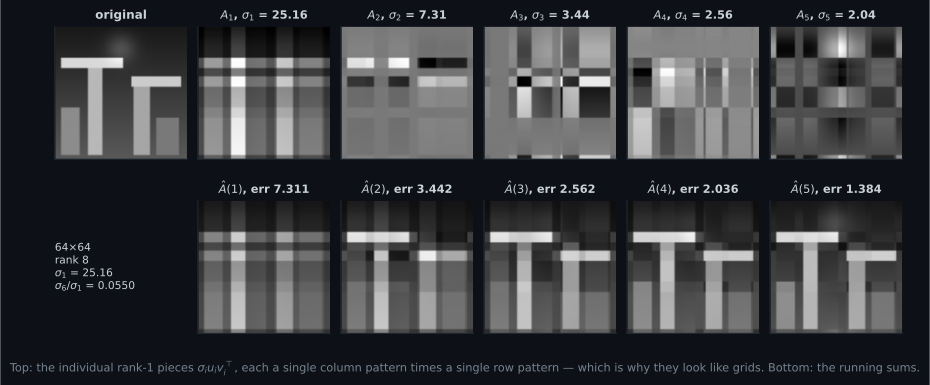
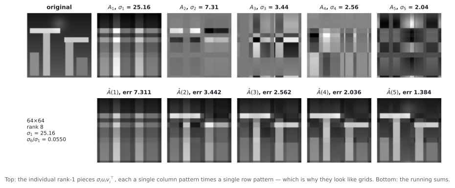
Reading the plot

From the rank-1 pieces figure. Look at the top row before the bottom row. Every panel has visible horizontal and vertical banding, and that is not an artefact — an outer product $\mathbf{u}\mathbf{v}^\top$ must look like that, because every row is a multiple of the same row pattern. This is the observation the book attaches to Figure 4.11, and seeing five of them side by side makes the point that a single rank-1 matrix cannot represent anything localised.

The bottom row is the sum. The energy table explains why it converges so fast:

$k$	cumulative share of squared energy
1	$88.96\%$
2	$96.47\%$
3	$98.13\%$
5	$99.64\%$
8	$100\%$ (exact)

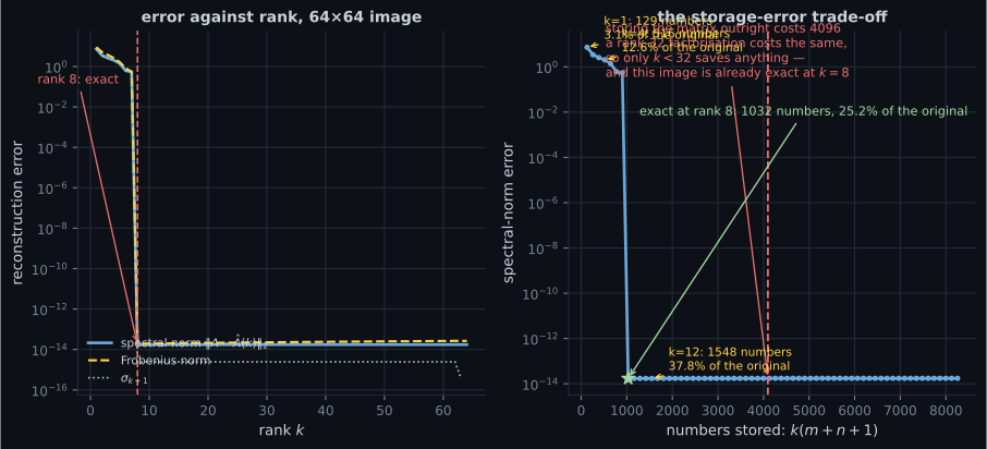
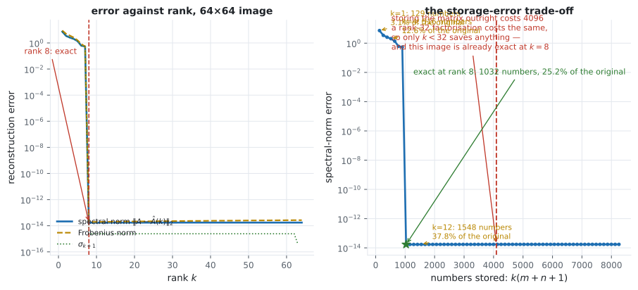
This image was built from a small number of rank-1 ingredients — a gradient, two rectangles, a blob — so it has exact rank 8 and a fast-decaying spectrum. Real photographs are not exactly low rank; they are approximately low rank, which is why the same procedure still works but never becomes exact.

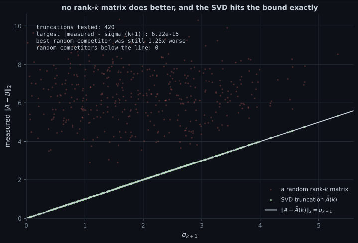
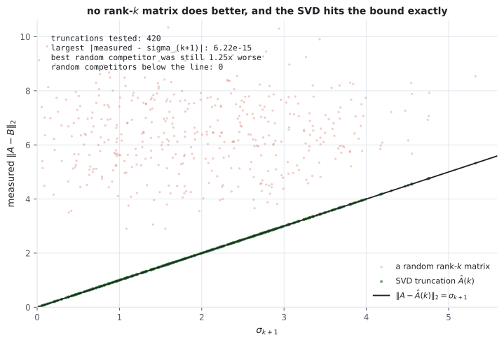
From the Eckart-Young figure. Two claims, two colours.

The green points test Equation 4.95. Over $420$ truncations the largest disagreement between the measured spectral error and $\sigma_{k+1}$ is $6.22\times10^{-15}$ — machine precision. The points are on the diagonal, and the word to notice is “on”: an inequality would have produced a cloud below the line.

The red points test Equation 4.94. Every one is a random rank-$k$ matrix, rescaled to the same Frobenius size as the truncation so the comparison is not rigged by magnitude. Zero of 420 landed below the line, and the best one was still $1.25\times$ worse. Random search does not find a better rank-$k$ matrix because there isn’t one.

From the compression figure. The left panel puts three curves on top of each other: the spectral error, the Frobenius error and $\sigma_{k+1}$. The spectral curve and the $\sigma_{k+1}$ curve are indistinguishable, which is Equation 4.95 again; the Frobenius curve sits slightly above, because it sums the whole tail rather than taking its largest element.

The right panel is the sober one, and it is the part the Stonehenge example can leave you over-optimistic about. A rank-$k$ factorisation of an $m \times n$ matrix costs $k(m+n+1)$ numbers, so it saves only when

$$k(m+n+1) < mn \quad\Longleftrightarrow\quad k < \frac{mn}{m+n+1}$$

For this $64\times64$ image that threshold is $k = 32$ — half the rank. For Stonehenge, $1432\times1910$, it is $k = 818$, so the book’s rank-5 approximation at $0.611\%$ is nowhere near it and the compression is genuine. The saving comes from the matrix being large and its useful rank being small, and it is the ratio that matters, not the rank. A $10\times10$ matrix of rank 3 costs $63$ numbers factored against $100$ stored — a saving, but a thin one.

Pitfalls

Eckart-Young is a statement about the spectral norm

Theorem 4.25 as the book states it minimises $\lVert\mathbf{A}-\mathbf{B}\rVert_2$. The same truncation also happens to minimise the Frobenius norm — that is the Mirsky/Schmidt extension, and the table above verifies it, with error $\sqrt{\sum_{i>k}\sigma_i^2}$ exactly. But it does not minimise every norm. For entrywise $\ell_1$ error, or for a weighted loss, or when entries are missing, the SVD truncation is not optimal and the problem is generally hard. Recommender systems with missing entries are exactly that harder problem, which is why they use iterative methods rather than a single SVD.

Low rank is not the same as few numbers

A rank-$k$ factorisation costs $k(m+n+1)$, so it saves nothing once $k \geq mn/(m+n+1)$ — for a square $n\times n$ matrix, roughly $n/2$. Measured on the $64\times64$ image above: break-even at $k=32$, and the exact factorisation at $k=8$ still costs $25.2\%$ of storing the matrix outright. Reporting “rank 8 out of 64” sounds like a $\smash{8/64}$ compression; it is a $\smash{1/4}$ one.

The singular values tell you where to truncate, but they do not tell you what to keep

Deciding $k$ from a scree plot is a judgement, not a theorem. Equation 4.95 tells you the error for each $k$; it does not tell you which error is acceptable, and a spectrum with no visible elbow — common for real data — gives you no guidance at all.

Truncation is a projection, and it discards signal along with noise

Denoising by truncation assumes the signal lives in the top singular directions and the noise in the bottom. When that is false — a faint but genuinely important feature, a rare class in a data matrix — truncation deletes it, and the error metric will look fine because that feature contributed little to the norm. Exercise 5 measures it: with a rank-3 signal and a small added patch, truncating at $k=3$ — the rank every energy criterion points at, $95.69\%$ of the squared energy — recovers only $7.3\%$ of the patch, while $k=4$ recovers $92.8\%$. Yet the overall Frobenius error is $7.3193$ at $k=3$ against $7.1801$ at $k=4$. The error metric cannot tell the two apart. Eckart-Young guarantees optimality with respect to a norm, and that is not the same as keeping what matters.

Rebuilding the approximation as a dense matrix throws away the benefit

(U[:, :k] * s[:k]) @ Vt[:k] gives you an $m\times n$ dense array again — the same memory as the original. Keep the factors. A matrix-vector product with the factored form costs $k(m+n)$ against $mn$, which is where the speed comes from as well as the space.

Do not compare singular values across differently scaled matrices

$\sigma$ scales linearly with the matrix, so "$\sigma_4 = 20\,232$" means nothing on its own — the Stonehenge $\sigma_1$ is about $228\,052$. Use ratios: $\sigma_{k+1}/\sigma_1$, or the cumulative share of $\sum\sigma_i^2$, both of which are scale-free.

Compare

how you might reduce a matrix’s rank	error in the spectral norm	optimal?
SVD truncation $\hat{\mathbf{A}}(k)$	exactly $\sigma_{k+1}$	yes, Theorem 4.25
keep the $k$ largest-magnitude entries	unbounded	no
keep the $k$ largest-norm rows	unbounded	no
a random rank-$k$ projection	typically much worse; measured best of 420 was $1.25\times$	no, but cheap and it comes with probabilistic bounds
a random rank-$k$ matrix	far worse	no
CUR / interpolative decomposition	within a factor of the optimum	no, but the factors are actual rows and columns, so they stay interpretable

The last row is the honest trade. Truncation is optimal but its factors are dense combinations of everything; CUR is slightly worse but every factor is a real row or column of your data.

pch.quizTag Check your understanding

1. Equation 4.95 says the error equals sigma-k-plus-one. Why is that nearly free once you have Theorem 4.24?

   A It requires a separate proof B Because A minus A-hat(k) is itself the tail of the SVD sum, so it is a matrix already in SVD form whose largest singular value is sigma-k-plus-one — and Theorem 4.24 says the spectral norm IS the largest singular value C Because the norms are equal by definition D Because the truncation is a projection
   pch.quizShowAnswer

   B — Because A minus A-hat(k) is itself the tail of the SVD sum, so it is a matrix already in SVD form whose largest singular value is sigma-k-plus-one — and Theorem 4.24 says the spectral norm IS the largest singular value — Equation 4.96 makes the difference explicit as the sum from k+1 to r. The hard half of Theorem 4.25 is the other one — Equation 4.94, optimality, which needs the rank-nullity contradiction.

2. The optimality argument reaches a contradiction by adding two dimensions. Which two, and what do they add up to?

   A The rank and the nullity of A, adding to n B The null space of B, which has dimension at least n-k, and the span of the first k+1 right-singular vectors, which has dimension k+1 — adding to n+1, so the two subspaces must share a nonzero vector C The row space and column space of A D The domain and codomain dimensions
   pch.quizShowAnswer

   B — The null space of B, which has dimension at least n-k, and the span of the first k+1 right-singular vectors, which has dimension k+1 — adding to n+1, so the two subspaces must share a nonzero vector — A vector in both would have to satisfy ||Ax|| < sigma-k-plus-one ||x|| from being in the null space of B, and ||Ax|| >= sigma-k-plus-one ||x|| from being in the singular-vector span. Chapter 2's rank-nullity theorem is what forbids it.

3. In 420 tests, zero random rank-k matrices beat the truncation and the best was 1.25 times worse. What does the 1.25 tell you that the zero does not?

   A Nothing extra B That the bound is not merely rarely violated but has real margin — random rank-k matrices are not even close, so the test is not just a near-tie decided by rounding C That the test needed more samples D That the truncation is 25 percent better on average
   pch.quizShowAnswer

   B — That the bound is not merely rarely violated but has real margin — random rank-k matrices are not even close, so the test is not just a near-tie decided by rounding — A best-competitor ratio of 1.0001 would have left it open whether the zero count was a floating-point artefact. At 1.25 the gap is unambiguous, and it is the closest of 420 attempts — the typical competitor is far worse.

4. The 64x64 image has exact rank 8. Why is that still only a 4-to-1 compression rather than 8-to-1?

   A Because the singular values must also be stored B Because a rank-k factorisation costs k(m+n+1) numbers, which is 8 times 129 equals 1032 against 4096 — the cost scales with m+n, not with n squared, so the saving depends on the ratio of k to mn/(m+n+1), which is 32 here C Because the reconstruction is not exact D Because the factors are dense
   pch.quizShowAnswer

   B — Because a rank-k factorisation costs k(m+n+1) numbers, which is 8 times 129 equals 1032 against 4096 — the cost scales with m+n, not with n squared, so the saving depends on the ratio of k to mn/(m+n+1), which is 32 here — This is why the book's Stonehenge example is so much more impressive: at 1432 by 1910 the break-even rank is 818, so rank 5 is a 0.611 percent cost. Big matrix, small useful rank.

5. Truncation minimises the spectral norm error. Where does that guarantee stop being the guarantee you want?

   A It never stops being enough B When entries are missing, when the loss is weighted or entrywise-L1, or when a faint feature matters more than its contribution to the norm — optimality with respect to a norm is not usefulness C Only for non-square matrices D Only when the rank is unknown
   pch.quizShowAnswer

   B — When entries are missing, when the loss is weighted or entrywise-L1, or when a faint feature matters more than its contribution to the norm — optimality with respect to a norm is not usefulness — Recommender systems are the standard example: with most entries unobserved the problem is no longer a single SVD and is generally hard, which is why iterative matrix-completion methods exist.

🧪 Try It Yourself

Exercise 1 – Eckart-Young at every k

pch.exerciseTag pch.exerciseTitle

Exercise 2 – The book’s Equation 4.100, and the slip in 4.101b

pch.exerciseTag pch.exerciseTitle

Exercise 3 – Nothing of rank k does better

pch.exerciseTag pch.exerciseTitle

Exercise 4 – When does a factorisation actually save anything?

pch.exerciseTag pch.exerciseTitle

Exercise 5 – Truncation as denoising, and where it fails

pch.exerciseTag pch.exerciseTitle

Recall card

• Any rank-r matrix is a weighted sum of r rank-1 outer products, A = sum of sigma-i u-i v-i-transpose, because Sigma is diagonal and pairs only matching singular vectors.
• An outer product looks like a grid: every row is a multiple of one row pattern, which is why a single rank-1 piece cannot represent anything localised.
• The rank-k approximation truncates that sum at k and has rank exactly k.
• The spectral norm is the largest stretch a matrix applies to any vector, and Theorem 4.24 says it equals sigma-1.
• Eckart-Young, Theorem 4.25, makes two claims: the truncation is the closest rank-k matrix in the spectral norm, and its error is exactly sigma-k-plus-one — equal to, not bounded by.
• Exactness is nearly free from Theorem 4.24, because the difference is itself the tail of the SVD sum; optimality is the hard half and rests on the rank-nullity theorem.
• Measured: over 420 truncations the error matched sigma-k-plus-one to 6.22e-15, and zero of 420 random rank-k competitors did better, the best being 1.25 times worse.
• The Frobenius error is the square root of the discarded tail of squared singular values, exactly — so the truncation is optimal in that norm too.
• Low rank is not the same as few numbers. A rank-k factorisation costs k(m+n+1), so it saves only for k below mn/(m+n+1) — 32 for a 64 by 64 matrix, 818 for the book’s 1432 by 1910 Stonehenge photograph.
• Optimality is with respect to a norm, not usefulness. With missing entries, a weighted loss, or a faint but important feature, the SVD truncation is no longer the right answer.

Next: Matrix Phylogeny — the family tree of every matrix class in this chapter, and which decomposition applies to each.