Actor-Critic and PPO (Intro)

Policy gradients ended with a working method and an unflattering number: REINFORCE’s baseline cut the gradient norm 35× and moved the final score by 0.27. Variance reduction that changes nothing is a strange result to leave standing.

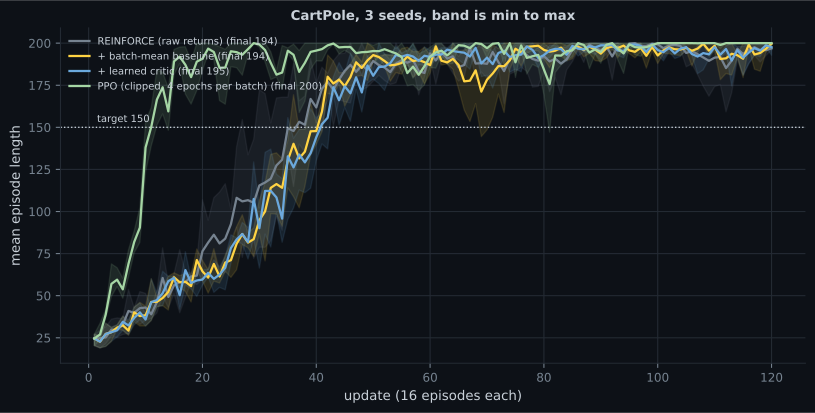
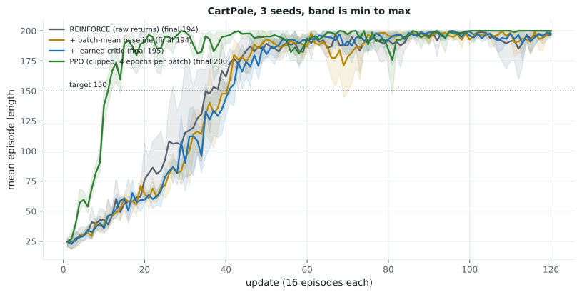
This page takes the two standard next steps and measures both. Actor-critic replaces the batch-mean baseline with a learned value function. PPO attacks a different axis entirely — not the variance of each update, but how many updates you can extract from each batch of experience.

One of them makes a large difference here and the other does not.

What you’ll learn

• Why a learned critic is a better baseline than a batch mean, and what it cost here.
• The PPO clipped objective derived, and what the ratio $r_t(\theta)$ actually measures.
• The measured result: 170 episodes to target against 544, a 3.2× sample-efficiency win.
• When the clip matters — measured by sweeping until it does.
• Why “PPO is more stable” is a claim about the worst seed, not the average.

The four methods

All on the same CartPole, the same 16-episode batches, the same 120 updates, three seeds each. The environment is the hand-written vectorised one from _rl.py; a random policy survives 23.09 steps and the episode cap is 200.

Method	Weight on each log-probability
REINFORCE	the raw discounted return $G_t$
+ batch-mean baseline	$(G_t - \bar{G}) / \sigma_G$
+ learned critic	$(G_t - V_\phi(s_t))$, whitened
PPO	the same advantage, but four clipped gradient steps per batch

figure CartPole, 3 seeds, band is min to max matplotlib

All four methods solve CartPole — final scores 193.9, 194.2, 195.0 and 199.9 — which is the first thing to say plainly. On a task this easy, the ranking by final score is nearly meaningless: the gap between best and worst is 6.0 against an episode cap of 200. What separates them is how fast they get there, and PPO's curve is the only one that is clearly different.

Method	Final score	Episodes to reach 150	Seeds solved	Seconds
REINFORCE (raw returns)	193.9	544	3/3	30.2
+ batch-mean baseline	194.2	624	3/3	35.7
+ learned critic	195.0	613	3/3	43.0
PPO (4 steps per batch)	199.9	170	3/3	52.4

The critic did not pay for itself here

A learned baseline scored 195.0 against the batch mean’s 194.2 and reached the target in 613 episodes against 624 — inside the noise, for 43.0 seconds against 35.7 and a second network to train. On CartPole the batch mean is already a good baseline, because episode returns within a batch are similar and the state-dependence a critic adds has little to predict. Reporting this as “actor-critic improves on REINFORCE” would be reading a 0.8 difference on a scale where the seeds spread further than that.

That leaves PPO, whose win is not on the score axis at all.

Sample efficiency is the axis that moved

figure 3 seeds each, mean over the seeds that reached the target matplotlib

PPO needed 170 episodes of environment interaction against REINFORCE's 544 — 3.2x fewer — while costing 1.7x the wall clock. That trade is the entire argument. On CartPole, where an episode costs microseconds, it is a bad trade; on a robot, a simulator that runs slower than real time, or anything where interaction is the expensive part, it is the only trade that matters.

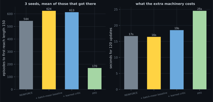
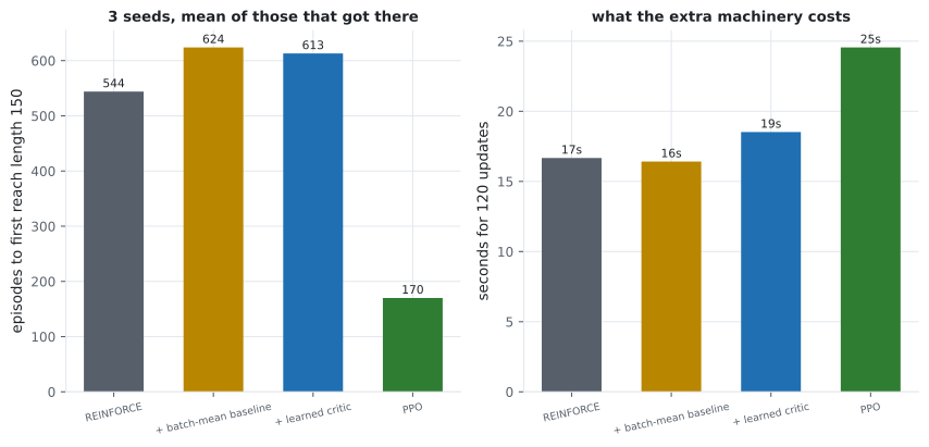
Every method here consumed exactly 1,920 episodes over 120 updates, because the batch size is fixed. The difference is where they were on the curve when they had spent 170 of them.

The mechanism is direct: REINFORCE takes one gradient step per batch and then throws the data away. PPO takes four. Four times the learning from the same experience, if the four steps are all valid — and the reason they are not all valid by default is the whole reason PPO exists.

Why you cannot just take four steps

The policy-gradient estimator is only correct for the policy that collected the data. After one gradient step the policy has changed, so the second step is computed on experience from a policy that no longer exists. PPO makes that explicit with a probability ratio:

$$r_t(\theta) = \frac{\pi_\theta(a_t \mid s_t)}{\pi_{\theta_{\text{old}}}(a_t \mid s_t)}$$

At the first gradient step $\theta = \theta_{\text{old}}$, so $r_t = 1$ exactly. As the steps accumulate, $r_t$ drifts away from 1 — and an advantage multiplied by a large ratio produces an enormous update justified by data the current policy would never have generated.

The clipped objective bounds that:

$$L^{\text{CLIP}}(\theta) = \mathbb{E}_t\left[\min\Bigl(r_t(\theta)\,\hat{A}_t,\; \operatorname{clip}\bigl(r_t(\theta),\, 1-\epsilon,\, 1+\epsilon\bigr)\,\hat{A}_t\Bigr)\right]$$

The $\min$ is what makes it a bound rather than a rescaling. When $\hat{A}_t > 0$ and the ratio has already climbed past $1 + \epsilon$, the clipped term is smaller and gets chosen — there is no further gradient for making an already-favoured action more likely. When $\hat{A}_t < 0$ and the ratio has fallen below $1 - \epsilon$, the same logic applies in reverse. Improvements outside the trust region are simply not counted.

python

ratio = tf.exp(log_probability - old_log)
clipped = tf.clip_by_value(ratio, 1 - clip, 1 + clip)
loss = -tf.reduce_mean(tf.minimum(ratio * advantages, clipped * advantages))

diagram Diagram mermaid

  flowchart TD
  C["collect 16 episodes
under policy theta_old"] --> S["store log pi_old(a|s)"]
  S --> L["step 1: ratio = 1 exactly"]
  L --> L2["step 2: ratio drifts"]
  L2 --> L3["step 3, 4, ... further still"]
  L3 --> Q{"bounded?"}
  Q -->|"clipped"| G["update capped at
1 +/- epsilon"]
  Q -->|"unclipped"| B["huge update justified by
data this policy never saw"]
  G --> C
  B --> F["worst seed: 9.2
below the random policy"]

When the clip actually matters

The obvious experiment is to remove the clip and watch PPO fail. It was run at the page’s default of four gradient steps per batch, and it did not fail: 199.9 with the clip against 199.4 without. That is a null result, and the reason is measurable — after four steps the policy has barely moved, so there is nothing for a trust region to bound.

So the sweep was extended until there was:

figure Same episode budget, only the number of gradient steps per batch changes matplotlib

At 1 and 4 steps the clip is measurably worthless — 198.3 against 198.3, and 199.9 against 199.4. At 16 it is the difference between 194.7 and 129.3, and the right panel shows where that average comes from: the unclipped worst seed scored 9.2, which is below the 23.09 a random policy gets. The clip does not make the average better; it stops one run in three from destroying itself.

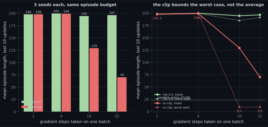
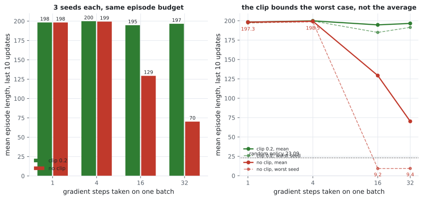
Gradient steps per batch	Clipped	Clipped, worst seed	Unclipped	Unclipped, worst seed
1	198.3	197.3	198.3	197.3
4	199.9	199.7	199.4	198.5
16	194.7	185.0	129.3	9.2
32	196.6	191.5	70.2	9.4

Three things worth stating precisely:

At one step the two are byte-for-byte equivalent. The ratio is exactly 1 for every sample, the clip never binds, and both columns read 198.3. That is a correctness check on the implementation as much as a result.

The failure is a variance failure. At 16 steps the unclipped mean of 129.3 is not three mediocre runs; it is two runs near 190 and one at 9.2 — worse than acting at random. The clip’s contribution is bounding the worst case, which is exactly what the word “proximal” is about and exactly what a mean-only report would hide.

More steps is not monotonically better even with the clip. 199.9 at four steps, 194.7 at sixteen, 196.6 at thirty-two. Past a point the extra steps are extracting increasingly stale signal, and the clip prevents disaster rather than delivering gains.

A drift measurement that did not work

The natural diagnostic is the share of samples whose ratio leaves the trust region, and it was measured: 0.0000, 0.0000, 0.0000 and 0.1325 at 1, 4, 16 and 32 steps. That column is nearly useless, and the reason is instructive — it is taken on the final batch of the run, and a policy that has already collapsed to near-deterministic produces ratios back near 1. The diagnostic only reports drift while learning is still happening, so it misses the exact runs it was meant to catch. The worst-seed column replaced it.

What actor-critic is still for

The critic earned nothing on CartPole, so it is worth being explicit about the condition under which it does, rather than leaving the impression that it never does.

A batch-mean baseline subtracts the same number from every state’s return. It therefore cannot express “this state was always going to score badly, so a below-average return here is not the action’s fault”. A learned $V_\phi(s)$ can. That distinction is worth nothing when all states in a batch have similar value — which on CartPole they do, since every non-terminal state is worth roughly the same — and worth a great deal when they do not, as in any task with distinct good and bad regions.

The measured cost of carrying it: 43.0 s against 35.7 s, a second network, and one more learning rate to get wrong.

sketch How far can one batch be reused? p5.js Pause Restart

Drag to set the gradient steps per batch, then toggle the clip. The bars are the measured mean and the worst of three seeds.

sketch The measured table, ranked p5.js Pause Restart

Click a column to rank every row by it. The bars are that column's values and the highest and lowest are computed from the numbers, not written in.

Pitfalls

• Reading the final scores. All four methods land between 193.9 and 199.9 on a task capped at 200. The ranking there is noise; the sample-efficiency column is the result.
• Claiming the critic helped. 195.0 against 194.2, for 43.0 s against 35.7 s and a second network. On CartPole it did not.
• Testing the clip at four steps. It measured 199.9 against 199.4 — a null result that would wrongly suggest the clip is decorative. It binds from 16 steps.
• Reporting only the mean when the failure is variance. Unclipped at 16 steps averages 129.3; its worst seed is 9.2, below random. Those are different findings.
• Assuming more reuse is better. 199.9 at 4 steps, 194.7 at 16, 196.6 at 32, even with the clip.
• Forgetting to store the old log-probabilities. $r_t$ needs $\pi_{\theta_{\text{old}}}$, captured before the first step. Recomputing it inside the loop makes every ratio exactly 1 and silently turns PPO back into repeated REINFORCE.
• Using model.predict in the rollout. ~470 ms per call against ~1.2 ms for a traced tf.function, and this page makes one call per environment frame.

Recap

• All four methods solved CartPole — 193.9, 194.2, 195.0 and 199.9 — so the final score separates nothing on this task.
• PPO reached mean length 150 in 170 episodes against REINFORCE’s 544, a 3.2× sample-efficiency win, for 1.7× the wall clock.
• The mechanism is reuse: four gradient steps per batch instead of one, made valid by bounding the probability ratio $r_t(\theta)$ inside $1 \pm 0.2$.
• A learned critic bought 0.8 points and 613 episodes against 624 — nothing, on a task where every state has roughly the same value. It is worth carrying where state values genuinely differ.
• The clip is worthless at 4 steps and decisive at 16: 194.7 against 129.3, with the unclipped worst seed at 9.2, below the random policy’s 23.09.
• At one gradient step per batch the clipped and unclipped runs are identical (198.3 both), because $r_t = 1$ exactly — which doubles as a correctness check.

Next

That is the reinforcement-learning phase. Phase 8 — Scaling & Deploying Deep Models turns to getting any of these models out of a notebook.

pch.quizTag pch.quizDefaultTitle

1. All four methods finished between 193.9 and 199.9 on a task capped at 200. What does that make the final-score column?

   A The main result B Nearly uninformative — the task is saturated, so the methods have to be separated on another axis, which here is episodes to reach the target C Evidence that PPO is best D A sign the environment is broken
   pch.quizShowAnswer

   B — Nearly uninformative — the task is saturated, so the methods have to be separated on another axis, which here is episodes to reach the target

2. Removing PPO's clip at four gradient steps per batch gave 199.4 against 199.9 — no measurable difference. Why?

   A The clip is decorative B After four steps the policy has barely moved from the one that collected the data, so the ratio stays near 1 and the trust region never binds C The clip was implemented incorrectly D CartPole is too simple for PPO
   pch.quizShowAnswer

   B — After four steps the policy has barely moved from the one that collected the data, so the ratio stays near 1 and the trust region never binds

3. Unclipped PPO at 16 steps averaged 129.3, with individual seeds at roughly 190, 190 and 9.2. What does the clip actually provide?

   A A higher average score B A bounded worst case — it stops one run in three from destroying itself, which is what 'proximal' refers to and what a mean-only report hides C Faster convergence D Lower memory use
   pch.quizShowAnswer

   B — A bounded worst case — it stops one run in three from destroying itself, which is what 'proximal' refers to and what a mean-only report hides

4. A learned critic scored 195.0 against a batch-mean baseline's 194.2, for 43.0 s against 35.7 s. Under what condition would the critic be worth it?

   A Always — a learned baseline is strictly better B When states in a batch have genuinely different values, so that a single subtracted number cannot express 'this state was always going to score badly' C When the learning rate is higher D When episodes are shorter
   pch.quizShowAnswer

   B — When states in a batch have genuinely different values, so that a single subtracted number cannot express 'this state was always going to score badly'

5. At one gradient step per batch, the clipped and unclipped runs both scored exactly 198.3. Why is that worth reporting?

   A It fills a row in the table B Because at one step r_t = 1 for every sample by construction, so the clip cannot bind — an identical result is a correctness check on the implementation C It shows one step is optimal D It proves the seeds were fixed correctly
   pch.quizShowAnswer

   B — Because at one step r_t = 1 for every sample by construction, so the clip cannot bind — an identical result is a correctness check on the implementation

6. What happens if you recompute the old log-probabilities inside the inner loop instead of storing them before the first step?

   A Nothing — it is equivalent B Every ratio becomes exactly 1, the clip never binds, and PPO silently degrades into taking several plain policy-gradient steps on stale data C The loss becomes negative D Training crashes
   pch.quizShowAnswer

   B — Every ratio becomes exactly 1, the clip never binds, and PPO silently degrades into taking several plain policy-gradient steps on stale data

🧪 Try It Yourself

pch.exerciseTag pch.exerciseTitle

pch.exerciseTag pch.exerciseTitle

pch.exerciseTag pch.exerciseTitle

pch.exerciseTag pch.exerciseTitle

pch.exerciseTag pch.exerciseTitle

pch.exerciseTag pch.exerciseTitle