Polynomial Regression

What you’ll learn

• why adding $x^2$ to the feature matrix lets a linear model fit a curve
• how to solve a quadratic fit by hand on five points
• how PolynomialFeatures explodes combinatorially, and how fast
• how to choose the degree with cross-validation and the one-standard-error rule
• how to read a learning curve to tell underfitting from overfitting
• why polynomial pipelines must scale their features

Intuition

A straight line through curved data is wrong in a specific, visible way: it misses low, then high, then low again. The residual plot shows a smile or a frown instead of a shapeless band.

The fix is disarmingly cheap. Do not change the algorithm — change the columns. Hand the model $x^2$ alongside $x$, and least squares will find the best parabola exactly the way it found the best line, because the model is still a weighted sum of whatever columns you supply. Linear regression is linear in the parameters, and never had an opinion about the features.

diagram Diagram mermaid

  flowchart LR
  X["Raw feature x"] --> PF["PolynomialFeatures(degree=2)"]
  PF --> C["Columns: x, x²"]
  C --> LR["The same LinearRegression"]
  LR --> Y["Curved prediction ŷ"]

The math

The model

A degree-$d$ polynomial in one feature:

$$\hat{y} = \theta_0 + \theta_1 x + \theta_2 x^2 + \cdots + \theta_d x^d$$

Rename $z_1 = x,\; z_2 = x^2,\; \ldots,\; z_d = x^d$ and it reads $\hat{y} = \theta_0 + \theta_1 z_1 + \cdots + \theta_d z_d$ — an ordinary multiple linear regression. The Normal Equation applies unchanged:

$$\boldsymbol{\theta} = (\mathbf{X}^\top\mathbf{X})^{-1}\mathbf{X}^\top\mathbf{y}, \qquad \mathbf{X} = \begin{bmatrix} 1 & x_1 & x_1^2 & \cdots & x_1^d \\ 1 & x_2 & x_2^2 & \cdots & x_2^d \\ \vdots & \vdots & \vdots & & \vdots \\ 1 & x_m & x_m^2 & \cdots & x_m^d \end{bmatrix}$$

That matrix has a name — the Vandermonde matrix — and a reputation: it becomes badly conditioned fast as $d$ grows, which is one reason high-degree fits misbehave numerically as well as statistically.

How many terms?

With $n$ input features and degree $d$, PolynomialFeatures generates every product of total degree at most $d$:

$$\text{number of terms} = \binom{n + d}{d}$$

features $n$	degree 2	degree 3	degree 5
1	3	4	6
3	10	20	56
10	66	286	3,003
100	5,151	176,851	≈ 96 million

Two features at degree 3 already give you interaction terms like $x_0^2 x_1$ — which is genuinely useful, and also how a tidy 10-column dataset becomes 286 columns without anyone deciding to do that.

Worked example by hand

Five points, $x$ chosen symmetric about zero so that $\sum x_i = 0$ and $\sum x_i^3 = 0$. That kills half the terms in $\mathbf{X}^\top\mathbf{X}$ and makes the algebra tractable.

$i$	$x_i$	$y_i$	$x_i^2$	$x_i y_i$	$x_i^2 y_i$
1	−2	9	4	−18	36
2	−1	4	1	−4	4
3	0	1	0	0	0
4	1	2	1	2	2
5	2	9	4	18	36
	0	25	10	−2	78

Step 1 — assemble the normal equations. With $\sum x = 0$, $\sum x^2 = 10$, $\sum x^3 = 0$ and $\sum x^4 = 34$:

$$\mathbf{X}^\top\mathbf{X} = \begin{bmatrix} 5 & 0 & 10 \\ 0 & 10 & 0 \\ 10 & 0 & 34 \end{bmatrix}, \qquad \mathbf{X}^\top\mathbf{y} = \begin{bmatrix} 25 \\ -2 \\ 78 \end{bmatrix}$$

Step 2 — the middle row is already solved. $10\theta_1 = -2$, so $\theta_1 = -0.2$.

Step 3 — solve the remaining 2×2 system.

$$5\theta_0 + 10\theta_2 = 25 \;\Longrightarrow\; \theta_0 = 5 - 2\theta_2$$

Substitute into $10\theta_0 + 34\theta_2 = 78$:

$$10(5 - 2\theta_2) + 34\theta_2 = 78 \;\Longrightarrow\; 14\theta_2 = 28 \;\Longrightarrow\; \theta_2 = 2,\quad \theta_0 = 1$$

The fitted curve is $\hat{y} = 1 - 0.2x + 2x^2$.

Step 4 — check.

$x_i$	$y_i$	$\hat{y}_i$	residual	squared
−2	9	9.4	−0.4	0.16
−1	4	3.2	+0.8	0.64
0	1	1.0	0.0	0.00
1	2	2.8	−0.8	0.64
2	9	8.6	+0.4	0.16
			0.0	1.60

$$\text{SST} = 58, \qquad R^2 = 1 - \frac{1.6}{58} \approx 0.972$$

Nothing here is new machinery. It is the Normal Equation from the previous page, applied to a design matrix that happens to contain a squared column.

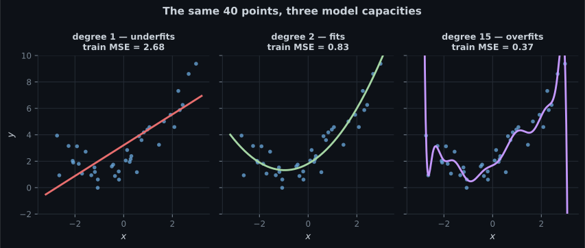
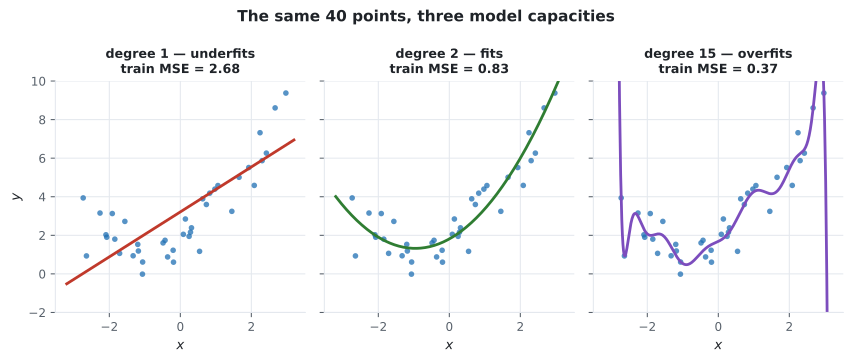
See it move

Three capacities cycling over the same curved dataset — watch the degree-12 curve chase individual points instead of the trend.

sketch Under and over-fitting a curved dataset p5.js Pause Restart

A degree-1 line underfits, a degree-2 curve fits well, and a high-degree polynomial overfits by wiggling through the noise. Click for a fresh sample.

figure The same 40 points, three model capacities matplotlib

Training MSE falls from 2.68 to 0.83 to 0.37 — and the model with the lowest training error is the one you would least want to deploy.

From scratch

Build the Vandermonde matrix explicitly and reuse the Normal Equation:

poly_from_scratch.py

import numpy as np
 
 
def vandermonde(x, degree):
    """Columns [1, x, x^2, ..., x^degree]."""
    x = np.asarray(x, dtype=float)
    return np.vstack([x**k for k in range(degree + 1)]).T
 
 
x = np.array([-2.0, -1.0, 0.0, 1.0, 2.0])
y = np.array([9.0, 4.0, 1.0, 2.0, 9.0])
 
X = vandermonde(x, 2)
print(X)
# [[ 1. -2.  4.]
#  [ 1. -1.  1.]
#  [ 1.  0.  0.]
#  [ 1.  1.  1.]
#  [ 1.  2.  4.]]
 
theta = np.linalg.solve(X.T @ X, X.T @ y)
print(theta.round(4))              # [ 1.  -0.2  2. ]
 
resid = y - X @ theta
print(resid.round(4))              # [-0.4  0.8  0.  -0.8  0.4]
print(round((resid ** 2).sum(), 4))  # 1.6

Same numbers as the hand calculation, including the residuals.

With scikit-learn

Never fit PolynomialFeatures outside a pipeline — the expansion has to be re-applied identically at prediction time, and the scaler after it has to be fitted on training data only:

poly_pipeline.py

import numpy as np
from sklearn.pipeline import make_pipeline
from sklearn.preprocessing import PolynomialFeatures, StandardScaler
from sklearn.linear_model import LinearRegression
 
rng = np.random.default_rng(7)
x = np.sort(rng.uniform(-3, 3, 120)).reshape(-1, 1)
y = 0.5 * x.ravel() ** 2 + x.ravel() + 2 + rng.normal(0, 1.1, 120)
 
model = make_pipeline(
    PolynomialFeatures(degree=2, include_bias=False),
    StandardScaler(),        # essential: x^5 dwarfs x, and scale wrecks conditioning
    LinearRegression(),
)
model.fit(x, y)
 
print(model.score(x, y).round(4))                   # 0.8196
print(model[0].get_feature_names_out())             # ['x0' 'x0^2']
print(model[-1].coef_.round(3))                     # [1.78  1.248]

include_bias=False matters: LinearRegression already fits an intercept, so leaving the constant column in gives you two intercepts and a rank-deficient design.

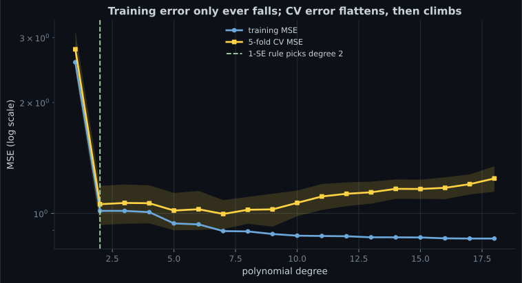
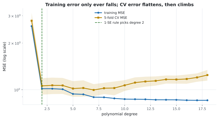
Choosing the degree

Training error falls forever as you add degrees. It has to — each extra term is a strictly larger family of curves. The only honest signal comes from data the model has not seen:

figure Training error versus cross-validated error by degree matplotlib

The CV curve is flat from degree 2 to about 10 — those models are statistically indistinguishable. The one-standard-error rule breaks the tie in favour of the simplest, degree 2.

Reading the plot

1. The cliff at degree 2 is the real signal. CV error drops from 2.79 to 1.06 and never improves meaningfully again. The data was generated by a quadratic, and the curve says so.
2. Degrees 2 through 10 are a tie. The shaded band is one standard error across folds; every point in that range sits inside it. Picking the exact minimum here would be reading noise.
3. The one-standard-error rule. Find the best CV score, add one standard error, and take the simplest model still under that threshold. Here it selects degree 2 — the right answer, and the one that generalises.
4. The gap after degree 10 is overfitting made visible. Training error keeps falling while CV error climbs.

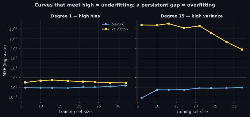
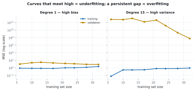
Learning curves

The degree curve varies capacity at fixed data. A learning curve does the opposite: fixed capacity, growing data. The two failure modes look completely different.

figure Learning curves for an underfitting and an overfitting model matplotlib

Curves that meet at a high error mean high bias — more data will not help. A wide persistent gap means high variance — more data will.

Symptom	Diagnosis	What actually helps
Both curves plateau high, close together	Underfitting (high bias)	More capacity: higher degree, more features
Training low, validation high, gap persists	Overfitting (high variance)	More data, lower degree, regularisation
Both low and converged	Good fit	Ship it

pch.algoTag Polynomial Regression Supervised · Regression

pch.algoApi sklearn.preprocessing.PolynomialFeatures + sklearn.linear_model.LinearRegression

pch.algoAssumes

• The relationship is smooth and can be approximated by a polynomial on the observed range
• Observations are independent
• Residual variance is constant

pch.algoCost

pch.algoTrain

O(m·p² + p³)

pch.algoPredict

O(p)

pch.algoMemory

O(p)

m = samples, p = expanded term count = binomial(n + d, d)

pch.algoHyperparams

• degree default 2 The one that matters. Choose by cross-validation, then take the simplest degree within one standard error of the best.
• include_bias default True Set False inside a pipeline whose final estimator already fits an intercept.
• interaction_only default False Keep cross terms like x0·x1 but drop pure powers — useful when you want interactions without curvature.

pch.algoReachFor

• A scatter plot or residual plot shows smooth curvature
• You have one to a handful of features and want to keep interpretability
• A physical relationship is genuinely quadratic or cubic

pch.algoLookElsewhere

• You have many features — the term count explodes combinatorially
• You need to predict outside the training range; polynomials diverge violently
• The curve has sharp kinks or steps — use splines or trees instead

Pitfalls

Always scale after expanding

With $x$ spanning 1 to 100, $x^5$ spans 1 to 10 billion. The design matrix becomes so badly conditioned that the solver returns nonsense. StandardScaler after PolynomialFeatures is not optional at degree 3 or above.

Polynomials extrapolate catastrophically

A degree-15 fit is close to the data inside its range and shoots to $\pm 10^6$ just outside it. Look at the third panel of the capacity figure: the curve leaves the plot at both ends. Never let a polynomial model see a feature value beyond the range it was trained on.

The term count is combinatorial, not linear

Ten features at degree 3 is 286 columns; at degree 5 it is 3,003. You will run out of samples before you run out of columns, and $n > m$ makes the least-squares solution non-unique.

Do not select the degree on the test set

Sweeping degrees and reporting the best test score is optimising against the test set — the number you report is no longer an estimate of anything. Select on cross-validation folds inside the training data, then touch the test set exactly once.

Compare

Approach	Shape it fits	Extrapolates	Cost with many features	Interpretability
Polynomial regression	Smooth global curve	Very badly	Explodes	Good at low degree
Splines	Smooth, piecewise, local	Poorly	Linear	Moderate
Decision tree	Steps	Flat (constant)	Linear	Moderate
Random forest	Smooth steps	Flat	Linear	Poor
Kernel ridge (RBF)	Smooth, local	Reverts to mean	Quadratic in samples	Poor
Log/sqrt transform	One fixed curve shape	Reasonably	Free	Very good

If the curvature is monotone, try transforming $y$ or $x$ with a log before reaching for a polynomial. One column, no degree to tune, and it extrapolates sensibly.

pch.quizTag pch.quizDefaultTitle

1. Why is polynomial regression still called a linear model?

   A Because the fitted curve is nearly straight over short ranges B Because it is linear in the parameters — x squared is just another column C Because it uses a straight line in a transformed space that must be recovered later D It is not; the name is a historical accident
   pch.quizShowAnswer

   B — Because it is linear in the parameters — x squared is just another column — Linearity refers to how the parameters enter the model. Treat x squared as a new feature and ordinary least squares applies with no modification.

2. Training MSE keeps falling as you raise the degree while CV MSE starts rising after degree 10. What is happening?

   A The optimiser is failing to converge B Overfitting: the extra capacity is fitting noise that does not generalise C The data needs rescaling D The cross-validation split is invalid
   pch.quizShowAnswer

   B — Overfitting: the extra capacity is fitting noise that does not generalise — Training error must fall with capacity. When held-out error turns upward, the extra flexibility is being spent memorising noise.

3. You have 10 features and set degree=3. Roughly how many columns does PolynomialFeatures produce?

   A 30 B 100 C 286 D 1000
   pch.quizShowAnswer

   C — 286 — The count is binomial(n + d, d) = binomial(13, 3) = 286, including the bias term. The growth is combinatorial, not linear.

4. Your CV curve is flat between degrees 2 and 10. Which degree should you ship?

   A Whichever has the exact lowest CV score B Degree 2 — the simplest model within one standard error of the best C Degree 10, for maximum flexibility D Average the predictions of all of them
   pch.quizShowAnswer

   B — Degree 2 — the simplest model within one standard error of the best — Differences inside one standard error are noise. The one-standard-error rule takes the simplest model that is statistically indistinguishable from the best, which is more likely to hold up on new data.

🧪 Try It Yourself

Exercise 1 – Expand features by hand

pch.exerciseTag pch.exerciseTitle

Exercise 2 – Solve the quadratic fit

pch.exerciseTag pch.exerciseTitle

Exercise 3 – Build a polynomial pipeline

pch.exerciseTag pch.exerciseTitle

Exercise 4 – Watch overfitting appear

pch.exerciseTag pch.exerciseTitle

Exercise 5 – Extrapolate and watch it explode

pch.exerciseTag pch.exerciseTitle

Recap

• Adding $x^2, x^3, \ldots$ as columns lets ordinary least squares fit curves — the model stays linear in its parameters.
• The hand-worked quadratic on five points gives $\hat{y} = 1 - 0.2x + 2x^2$ with $R^2 = 0.972$.
• PolynomialFeatures produces $\binom{n+d}{d}$ terms; 10 features at degree 3 is 286 columns.
• Choose the degree with cross-validation, then apply the one-standard-error rule to prefer the simplest model in the tie.
• Learning curves distinguish the two failure modes: converged-and-high is bias, wide-gap is variance.
• Scale after expanding, and never extrapolate.

Exercise 6 – Apply the one-standard-error rule

pch.exerciseTag pch.exerciseTitle

Next

Continue to Cost Functions - Mean Squared Error (MSE) — a closer look at the loss every fit on this page was silently minimising, and what changes when you pick a different one.