Logistic Regression (Binary vs Multiclass)

What you’ll learn

why a classifier is named “regression”, and what it is actually regressing
the sigmoid derived from log-odds, not pulled out of the air
log loss, why it is convex, and why it punishes confident mistakes so harshly
a full gradient step computed by hand on four rows
softmax regression for more than two classes, and why it is not the same as multilabel
how moving the threshold trades precision against recall on a real dataset

Intuition

A linear model outputs any real number. A probability has to live between 0 and 1. Logistic regression is the smallest possible bridge between the two: compute the linear score exactly as in Phase 3, then squash it.

The squashing function is not arbitrary. Ask instead: what quantity can a linear model predict without bounds? The answer is the log-odds. Odds run from 0 to infinity; their logarithm runs from $-\infty$ to $+\infty$ — exactly the range a linear model produces. So model the log-odds linearly, then invert to recover the probability. The inverse is the sigmoid.

diagram Diagram mermaid

  flowchart LR
  X["Features x"] --> Z["Linear score
z = w·x + b"]
  Z --> S["Sigmoid
p = 1 / (1 + e^-z)"]
  S --> P["Probability p"]
  P --> T["Threshold (default 0.5)"]
  T --> Y["Predicted class"]

The math

From odds to the sigmoid

For a probability $p$ , the odds are $p/(1-p)$ and the log-odds (or logit) are their logarithm. Model that linearly:

\operatorname{logit}(p) = \log\frac{p}{1-p} = \mathbf{w}^\top\mathbf{x} + b = z

Solve for $p$ :

\frac{p}{1-p} = e^{z} \;\Longrightarrow\; p = e^{z} - p\,e^{z} \;\Longrightarrow\; p\left(1 + e^{z}\right) = e^{z} \;\Longrightarrow\; p = \frac{e^{z}}{1 + e^{z}} = \frac{1}{1 + e^{-z}}

\boxed{\;\sigma(z) = \frac{1}{1 + e^{-z}}\;}

The sigmoid is not a design choice; it is what you get by insisting that a linear model predicts log-odds. This also hands you the interpretation of a coefficient: $w_j$ is the change in log-odds per unit of $x_j$ , so $e^{w_j}$ is the multiplicative change in the odds.

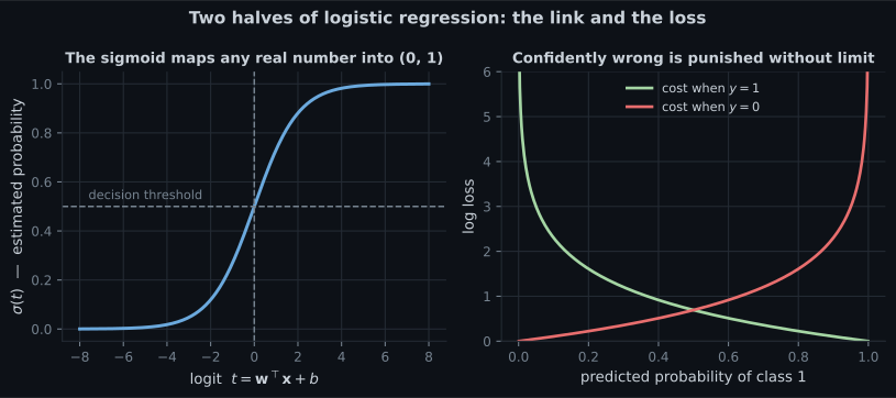
Log loss

Squared error against a sigmoid output is non-convex, so gradient descent could get stuck. Instead use the negative log-likelihood of a Bernoulli outcome:

J(\mathbf{w}, b) = -\frac{1}{m}\sum_{i=1}^{m}\left[ y^{(i)}\log p^{(i)} + \left(1 - y^{(i)}\right)\log\left(1 - p^{(i)}\right) \right]

Only one term is ever active per row: if $y = 1$ the cost is $-\log p$ , if $y = 0$ it is $-\log(1-p)$ . Both blow up as the model becomes confidently wrong.

Left panel: the sigmoid curve rising from 0 to 1 through 0.5 at z equals zero. Right panel: two log loss curves, one exploding as the predicted probability approaches zero and the other as it approaches one. — Predicting 0.01 for a true positive costs 4.6; predicting 0.5 costs 0.69. Log loss makes overconfidence far more expensive than uncertainty.

The gradient — the surprise

Differentiate log loss with respect to the weights and, after the algebra cancels, you get:

\frac{\partial J}{\partial w_j} = \frac{1}{m}\sum_{i=1}^{m}\left(p^{(i)} - y^{(i)}\right)x_j^{(i)}

That is exactly the linear regression gradient, with the prediction replaced by the sigmoid output. The messy $\sigma'(z) = \sigma(z)(1-\sigma(z))$ term produced by the chain rule cancels against the derivative of the logarithm. Log loss is the loss that makes logistic regression as simple to optimise as least squares — a strong argument that it is the right loss, not merely a convenient one.

There is no closed form, but $J$ is convex in $(\mathbf{w}, b)$ , so gradient descent always reaches the global minimum.

Worked example by hand

Four emails, one feature: the number of links. Start from $w = 1.0$ , $b = -2.5$ .

$i$	links $x$	true $y$	$z = x - 2.5$	$p = \sigma(z)$	loss
1	1	0	−1.5	0.1824	$-\log(0.8176) = 0.2014$
2	2	0	−0.5	0.3775	$-\log(0.6225) = 0.4741$
3	3	1	+0.5	0.6225	$-\log(0.6225) = 0.4741$
4	4	1	+1.5	0.8176	$-\log(0.8176) = 0.2014$

Step 1 — the cost.

J = \frac{0.2014 + 0.4741 + 0.4741 + 0.2014}{4} = 0.3377

Step 2 — the errors $p - y$ .

p - y = [\,0.1824,\; 0.3775,\; -0.3775,\; -0.1824\,]

Step 3 — the gradients.

\frac{\partial J}{\partial w} = \frac{1}{4}\Big[(0.1824)(1) + (0.3775)(2) + (-0.3775)(3) + (-0.1824)(4)\Big] = -0.2312

\frac{\partial J}{\partial b} = \frac{0.1824 + 0.3775 - 0.3775 - 0.1824}{4} = 0.0000

Step 4 — one step at $\alpha = 1$ .

w \leftarrow 1.0 - (1)(-0.2312) = 1.2312, \qquad b \leftarrow -2.5 - (1)(0) = -2.5

The intercept gradient is exactly zero because the data is symmetric about $x = 2.5$ , which is where $b = -2.5$ already places the boundary. Only the slope needs to grow — the model is being told to become more confident, not to move the boundary. Left running, $w$ diverges toward infinity, because perfectly separable data has no finite maximum-likelihood solution. Regularisation is what stops that, which is why scikit-learn applies an $\ell_2$ penalty by default.

See it move

sketch The sigmoid curve p5.js

As the linear score z moves left to right, the sigmoid squashes it into a probability between 0 and 1; the dot traces the current point and its probability.

From scratch

logistic_from_scratch.py

import numpy as np
 
 
def sigmoid(z):
    return 1 / (1 + np.exp(-z))
 
 
def log_loss(y, p, eps=1e-15):
    p = np.clip(p, eps, 1 - eps)          # never take log(0)
    return float(-(y * np.log(p) + (1 - y) * np.log(1 - p)).mean())
 
 
x = np.array([1.0, 2.0, 3.0, 4.0])
y = np.array([0.0, 0.0, 1.0, 1.0])
w, b = 1.0, -2.5
 
p = sigmoid(w * x + b)
print(p.round(4))                     # [0.1824 0.3775 0.6225 0.8176]
print(round(log_loss(y, p), 4))       # 0.3377
 
grad_w = float(((p - y) * x).mean())
grad_b = float((p - y).mean())
print(round(grad_w, 4), round(grad_b, 4))   # -0.2312 0.0
 
w, b = w - 1.0 * grad_w, b - 1.0 * grad_b
print(round(w, 4), round(b, 4))             # 1.2312 -2.5
print(round(log_loss(y, sigmoid(w * x + b)), 4))   # 0.318 — the cost fell

logistic_from_scratch.py

import numpy as np
 
 
def sigmoid(z):
    return 1 / (1 + np.exp(-z))
 
 
def log_loss(y, p, eps=1e-15):
    p = np.clip(p, eps, 1 - eps)          # never take log(0)
    return float(-(y * np.log(p) + (1 - y) * np.log(1 - p)).mean())
 
 
x = np.array([1.0, 2.0, 3.0, 4.0])
y = np.array([0.0, 0.0, 1.0, 1.0])
w, b = 1.0, -2.5
 
p = sigmoid(w * x + b)
print(p.round(4))                     # [0.1824 0.3775 0.6225 0.8176]
print(round(log_loss(y, p), 4))       # 0.3377
 
grad_w = float(((p - y) * x).mean())
grad_b = float((p - y).mean())
print(round(grad_w, 4), round(grad_b, 4))   # -0.2312 0.0
 
w, b = w - 1.0 * grad_w, b - 1.0 * grad_b
print(round(w, 4), round(b, 4))             # 1.2312 -2.5
print(round(log_loss(y, sigmoid(w * x + b)), 4))   # 0.318 — the cost fell

Every figure matches the hand calculation, and the cost drops from 0.3377 to 0.3180 in one step.

With scikit-learn

Binary: one feature, one boundary

iris_binary.py

import numpy as np
from sklearn.datasets import load_iris
from sklearn.linear_model import LogisticRegression
 
iris = load_iris()
X = iris.data[:, 3:]                      # petal width only
y = (iris.target == 2).astype(int)        # 1 if Iris virginica
 
model = LogisticRegression().fit(X, y)
 
print(model.predict([[1.7], [1.5]]))          # [1 0]
print(model.predict_proba([[2.0]]).round(3))  # [[0.187 0.813]]
 
boundary = -model.intercept_[0] / model.coef_[0][0]
print(f"p = 0.5 at petal width {boundary:.4f} cm")   # 1.6603 cm

iris_binary.py

import numpy as np
from sklearn.datasets import load_iris
from sklearn.linear_model import LogisticRegression
 
iris = load_iris()
X = iris.data[:, 3:]                      # petal width only
y = (iris.target == 2).astype(int)        # 1 if Iris virginica
 
model = LogisticRegression().fit(X, y)
 
print(model.predict([[1.7], [1.5]]))          # [1 0]
print(model.predict_proba([[2.0]]).round(3))  # [[0.187 0.813]]
 
boundary = -model.intercept_[0] / model.coef_[0][0]
print(f"p = 0.5 at petal width {boundary:.4f} cm")   # 1.6603 cm

The boundary is where $z = 0$ , so $x = -b/w$ — a number you can read off the coefficients directly and quote to a botanist.

Multiclass: softmax regression

For $k$ classes the model computes one score per class and normalises them:

p_k = \frac{\exp(s_k(\mathbf{x}))}{\sum_{j=1}^{K}\exp(s_j(\mathbf{x}))}, \qquad s_k(\mathbf{x}) = \mathbf{w}_k^\top\mathbf{x} + b_k

The predicted class is $\arg\max_k p_k$ , and the loss generalises to cross entropy, which reduces to ordinary log loss when $K = 2$ .

iris_softmax.py

from sklearn.datasets import load_iris
from sklearn.linear_model import LogisticRegression
 
iris = load_iris()
X = iris.data[:, (2, 3)]                  # petal length, petal width
y = iris.target                           # three classes
 
model = LogisticRegression(C=10, max_iter=1000).fit(X, y)
 
print(model.predict([[5, 2]]))                  # [2]  -> virginica
print(model.predict_proba([[5, 2]]).round(3))   # [[0.    0.057 0.943]]
print(f"training accuracy {model.score(X, y):.4f}")   # 0.9600

iris_softmax.py

from sklearn.datasets import load_iris
from sklearn.linear_model import LogisticRegression
 
iris = load_iris()
X = iris.data[:, (2, 3)]                  # petal length, petal width
y = iris.target                           # three classes
 
model = LogisticRegression(C=10, max_iter=1000).fit(X, y)
 
print(model.predict([[5, 2]]))                  # [2]  -> virginica
print(model.predict_proba([[5, 2]]).round(3))   # [[0.    0.057 0.943]]
print(f"training accuracy {model.score(X, y):.4f}")   # 0.9600

Scatter of iris petal length against petal width coloured by species, with three shaded regions separated by two straight decision boundaries. — Each boundary is straight, because each class score is linear. Setosa separates perfectly; versicolor and virginica overlap slightly, which is where the remaining 4% of errors live.

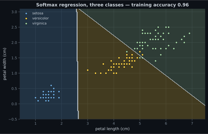
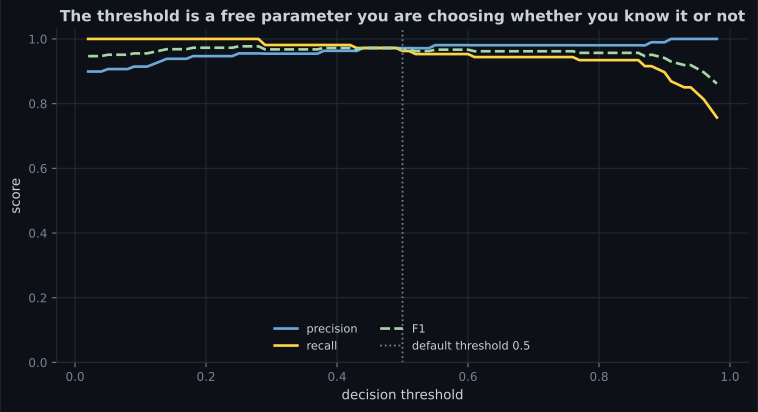
Choosing the threshold

predict()predict() uses 0.5. Nothing about your problem chose that number.

Precision, recall and F1 plotted against the decision threshold from 0.02 to 0.98. Precision rises toward 1 as the threshold increases while recall falls, and F1 peaks somewhere in between. — One trained model, no retraining. Sliding the threshold from 0.1 to 0.9 moves precision from 0.82 to 1.00 and recall from 0.98 to 0.88.

Reading the plot

Threshold	Precision	Recall	F1	When you would pick it
0.1	0.818	0.984	0.894	Screening — missing a case is unacceptable
0.3	0.859	0.953	0.904	Cautious triage
0.5	0.938	0.938	0.938	The default, balanced here by coincidence
0.7	1.000	0.922	0.959	Automated action — a false alarm is costly
0.9	1.000	0.875	0.933	Only act on near-certainty

On this dataset the best F1 comes from 0.7, not 0.5. That is a free improvement, available from a model that was already trained.

algorithmLogistic RegressionSupervised · Classification · Linear

APIsklearn.linear_model.LogisticRegression

Assumes

Log-odds of the positive class are linear in the features
Observations are independent
Little or no perfect multicollinearity
Enough samples per feature — roughly 10 events per predictor is the usual rule

Cost

train: O(m·n·i)
predict: O(n)
memory: O(n)

m = samples, n = features, i = solver iterations

Hyperparameters that matter

Cdefault 1.0INVERSE regularisation strength — smaller C means a stronger penalty. The opposite of alpha elsewhere in scikit-learn.
penaltydefault l2'l1' produces sparse coefficients (needs solver='liblinear' or 'saga'); 'elasticnet' needs 'saga'.
class_weightdefault None'balanced' reweights the loss by inverse class frequency — the first thing to try on imbalanced data.
max_iterdefault 100Raise it when you see a ConvergenceWarning; unscaled features are the usual cause.
solverdefault lbfgs'saga' for large or sparse data and L1; 'liblinear' for small binary problems.

Reach for it when

You need calibrated probabilities, not just labels
You must explain each feature's effect as a change in odds
You want a fast, strong baseline before trying anything complex
The classes are close to linearly separable in your feature space

Look elsewhere when

The boundary is genuinely non-linear and you cannot engineer the features
Features vastly outnumber samples without regularisation
You need to model complex feature interactions automatically — use a tree ensemble

Pitfalls

Compare

Model	Outputs probability	Boundary	Handles non-linearity	Interpretability
Logistic Regression	Yes, calibrated	Linear	Only via engineered features	Very high — odds ratios
Linear SVM	No (needs Platt scaling)	Linear, max-margin	Via kernels	Moderate
KNN	Yes, but coarse	Local	Naturally	Low
Naive Bayes	Yes, poorly calibrated	Quadratic-ish	Limited	Moderate
Decision Tree	Yes, coarse	Axis-aligned steps	Naturally	High for small trees
Gradient Boosting	Yes, needs calibration	Complex	Naturally	Low

quizCheck yourself

Why is the sigmoid the right function to squash a linear score into a probability?
Show answer
B — It is the inverse of the logit, so modelling log-odds linearly produces it automatically — Log-odds range over all real numbers, which is exactly what a linear model outputs. Inverting the logit to recover the probability gives the sigmoid — it is derived, not chosen.
What is remarkable about the gradient of log loss for logistic regression?
Show answer
B — It is identical in shape to the linear regression gradient: the mean of (prediction minus target) times the feature — The sigmoid derivative cancels against the log derivative, leaving the same clean expression as least squares. That cancellation is a strong hint log loss is the natural pairing for the sigmoid.
In LogisticRegression, what does a small value of C mean?
Show answer
B — Strong regularisation, because C is the inverse of the penalty strength — C is the inverse of regularisation strength, the reverse of the alpha convention used by Ridge and Lasso. C = 0.01 penalises heavily; C = 100 barely penalises at all.
Your model's best F1 occurs at a threshold of 0.7 rather than 0.5. What should you do?
Show answer
B — Use 0.7 — the threshold is a free parameter applied after training, and no retraining is needed — predict() simply compares predict_proba() against 0.5. Comparing against 0.7 instead is a one-line change that costs nothing and improves the metric you care about.

🧪 Try It Yourself

Exercise 1 – Implement the sigmoid

Exercise 2 – Compute log loss by hand

Exercise 3 – One gradient step

Exercise 4 – Read the decision boundary off the coefficients

Exercise 5 – Move the threshold, change the metrics

Recap

Model the log-odds linearly and invert; the sigmoid falls out of the algebra.
Log loss is the negative Bernoulli log-likelihood, convex, and it punishes confident errors without limit.
Its gradient is $\frac{1}{m}\sum(p - y)x$ — the same shape as least squares, because the sigmoid and log derivatives cancel.
Hand-worked on four rows: cost 0.3377, $\partial J/\partial w = -0.2312$ , $\partial J/\partial b = 0$ .
Softmax extends to $K$ mutually exclusive classes; independent sigmoids handle multilabel.
The threshold is a post-training decision. On the breast-cancer model it moves precision from 0.82 to 1.00 while recall falls from 0.98 to 0.88.
CC is the inverse of regularisation strength, and features must be scaled.

Exercise 6 – Read a coefficient as an odds ratio

Continue to K-Nearest Neighbors (KNN) — a classifier with no training step at all, that decides purely by looking at whoever is closest.

If this helped you, consider buying me a coffee ☕

Buy me a coffee