Basis and Rank

§2.5 asked which vectors in a pile are redundant. This section asks the two follow-up questions that matter: what is the smallest set that still builds everything, and how many vectors is that?

The answers are the basis and the rank, and the rank turns out to be the single most informative number you can extract from a matrix. It decides invertibility, solvability, the dimension of the image, the dimension of the null space, and — once §4.6 arrives — how well the matrix can be compressed.

What you’ll learn

• Generating set, span, and what makes a generating set minimal.
• Four equivalent ways to say “basis”, and why the fourth one (unique coordinates) is the useful one.
• Why every basis of a space has the same size, which is what makes dimension well defined.
• Rank, and the six properties of it that do all the work.
• Why a basis is not unique but the rank is — and how to find a basis of a subspace in three steps.

Intuition: describing any location in a city

Take a city on a grid. “Three blocks east, two blocks north” locates anything. Two directions are enough, and neither is redundant — drop “north” and the whole northern half of the city becomes unreachable.

That pair is a basis: enough to reach everything (a generating set), with nothing to spare (linearly independent). Add “four blocks north-east” as a third direction and you still reach everything, but the set is no longer minimal — the description of a location stops being unique, because you can now get there in more than one way.

Uniqueness is what you buy by insisting on minimality, and it is the whole reason bases matter.

diagram Diagram mermaid

  flowchart TD
  A["a set of vectors"] --> S["SPAN: everything
they can build"]
  S --> Q1{"does the span
cover all of V?"}
  Q1 -->|"no"| NG["not a generating set"]
  Q1 -->|"yes"| GS["GENERATING SET"]
  GS --> Q2{"is it minimal?
equivalently: independent?"}
  Q2 -->|"no"| RED["redundant — coordinates
are NOT unique"]
  Q2 -->|"yes"| BAS["BASIS"]
  BAS --> D["its size is the DIMENSION,
the same for every basis"]
  BAS --> U["every vector has EXACTLY ONE
coordinate representation"]

The math

Generating set and span

Given a vector space $V$ and a set $\mathcal{A} = \{\mathbf{x}_1,\dots,\mathbf{x}_k\} \subseteq \mathcal{V}$:

• If every $\mathbf{v} \in \mathcal{V}$ can be written as a linear combination of $\mathbf{x}_1,\dots,\mathbf{x}_k$, then $\mathcal{A}$ is a generating set of $V$.
• The set of all linear combinations of vectors in $\mathcal{A}$ is the span of $\mathcal{A}$.
• If $\mathcal{A}$ spans $V$ we write $V = \operatorname{span}[\mathcal{A}]$, or $V = \operatorname{span}[\mathbf{x}_1,\dots,\mathbf{x}_k]$.

The span is always a subspace — it contains $\mathbf{0}$ (all coefficients zero) and it is closed under both operations by construction. So “span” is the standard way to manufacture a subspace, and §2.4’s closing remark said every subspace arises this way.

Basis

A generating set $\mathcal{A}$ of $V$ is minimal if there is no smaller set $\tilde{\mathcal{A}} \subsetneq \mathcal{A}$ that still spans $V$. Every linearly independent generating set is minimal, and is called a basis of $V$.

The book then gives four equivalent characterisations, and they are worth knowing as a group because different problems make different ones easy to check. For $\mathcal{B} \subseteq \mathcal{V}$ nonempty, these are the same statement:

1. $\mathcal{B}$ is a basis of $V$.
2. $\mathcal{B}$ is a minimal generating set.
3. $\mathcal{B}$ is a maximal linearly independent set — adding any other vector of $V$ makes it dependent.
4. Every $\mathbf{x} \in V$ is a linear combination of vectors from $\mathcal{B}$, and that combination is unique:

$$\mathbf{x} = \sum_{i=1}^{k}\lambda_i\mathbf{b}_i = \sum_{i=1}^{k}\psi_i\mathbf{b}_i \quad\Longrightarrow\quad \lambda_i = \psi_i \text{ for all } i$$

Characterisation 3 is the sharpest framing: a basis is squeezed from both sides. Too few vectors and it does not span; too many and it is dependent. It sits exactly at the boundary — minimal among spanning sets and maximal among independent sets at the same time.

Characterisation 4 is the one you actually use. Unique coordinates are what make “the coordinates of $\mathbf{x}$” a well-defined phrase, and §2.7 builds the entire transformation-matrix machinery on top of it.

Why uniqueness follows from independence

One line, and it is the reason the two conditions are the same. Suppose $\sum_i\lambda_i\mathbf{b}_i = \sum_i\psi_i\mathbf{b}_i$. Subtracting,

$$\sum_{i}(\lambda_i - \psi_i)\mathbf{b}_i = \mathbf{0}$$

Independence says the only combination reaching zero is the trivial one, so every $\lambda_i - \psi_i = 0$. Uniqueness of coordinates is linear independence, rewritten.

Dimension

Every vector space has a basis, and there are many of them — no basis is unique. But all of them have the same number of elements, and that number is the dimension $\dim(V)$.

That invariance is what makes dimension meaningful, and it is not obvious. Two people can pick totally different bases of $\mathbb{R}^3$ and both will have exactly three vectors.

For a subspace $U \subseteq V$: $\dim(U) \le \dim(V)$, with equality if and only if $U = V$. So a proper subspace is always strictly lower dimensional — there is no “same-dimension proper subspace”.

Dimension is not the number of entries in a vector

The book’s own remark, and a genuine trap. The space $V = \operatorname{span}\!\left[\begin{bmatrix}0\\1\end{bmatrix}\right]$ is one-dimensional, even though its single basis vector has two components.

Dimension counts independent directions, not coordinates. A line in $\mathbb{R}^{1000}$ is one-dimensional. This is exactly the confusion Chapter 10 exists to exploit: data living in $\mathbb{R}^{1000}$ often occupies a subspace of dimension 20, and PCA finds it.

Finding a basis of a subspace

Three steps, and the book states them as a recipe. For $U = \operatorname{span}[\mathbf{x}_1,\dots,\mathbf{x}_m] \subseteq \mathbb{R}^n$:

1. Write the spanning vectors as the columns of a matrix $\mathbf{A}$.
2. Determine the row-echelon form of $\mathbf{A}$.
3. The spanning vectors belonging to the pivot columns are a basis of $U$.

This is §2.5’s independence test, reused verbatim. Same computation, different question: there we asked whether the set was independent, here we ask which subset is.

Rank

The number of linearly independent columns of $\mathbf{A} \in \mathbb{R}^{m\times n}$ equals the number of linearly independent rows, and that common number is the rank, $\operatorname{rk}(\mathbf{A})$.

That equality is remarkable and easy to skate past. There is no obvious reason a matrix should have as many independent rows as columns — the two counts are about different vectors living in different spaces — and yet they always agree.

The six properties that do the work:

property	statement
row rank = column rank	$\operatorname{rk}(\mathbf{A}) = \operatorname{rk}(\mathbf{A}^\top)$
image dimension	the columns span a subspace $U \subseteq \mathbb{R}^m$ with $\dim(U) = \operatorname{rk}(\mathbf{A})$; this is the image or range
row space dimension	the rows span $W \subseteq \mathbb{R}^n$ with $\dim(W) = \operatorname{rk}(\mathbf{A})$
invertibility	$\mathbf{A} \in \mathbb{R}^{n\times n}$ is invertible iff $\operatorname{rk}(\mathbf{A}) = n$
solvability	$\mathbf{A}\mathbf{x} = \mathbf{b}$ is solvable iff $\operatorname{rk}(\mathbf{A}) = \operatorname{rk}(\mathbf{A}\mid\mathbf{b})$
null-space dimension	the solutions of $\mathbf{A}\mathbf{x} = \mathbf{0}$ form a subspace of dimension $n - \operatorname{rk}(\mathbf{A})$

A matrix has full rank when $\operatorname{rk}(\mathbf{A}) = \min(m, n)$ — the largest possible for its shape — and is rank deficient otherwise.

The solvability property is the one §2.1’s classification code used, and the null-space property is where §2.3’s free-variable count came from. Both were stated there and are proved here.

Worked example by hand

The book’s Example 2.17. Find a basis of the subspace $U \subseteq \mathbb{R}^5$ spanned by

$$\mathbf{x}_1 = \begin{bmatrix}1\\2\\-1\\-1\\-1\end{bmatrix},\; \mathbf{x}_2 = \begin{bmatrix}2\\-1\\1\\2\\-2\end{bmatrix},\; \mathbf{x}_3 = \begin{bmatrix}3\\-4\\3\\5\\-3\end{bmatrix},\; \mathbf{x}_4 = \begin{bmatrix}-1\\8\\-5\\-6\\1\end{bmatrix}$$

Write them as columns and reduce:

$$\begin{bmatrix} 1 & 2 & 3 & -1\\ 2 & -1 & -4 & 8\\ -1 & 1 & 3 & -5\\ -1 & 2 & 5 & -6\\ -1 & -2 & -3 & 1 \end{bmatrix} \;\rightsquigarrow\; \begin{bmatrix} 1 & 2 & 3 & -1\\ 0 & 1 & 2 & -2\\ 0 & 0 & 0 & 1\\ 0 & 0 & 0 & 0\\ 0 & 0 & 0 & 0 \end{bmatrix}$$

Pivots sit in columns 1, 2 and 4. So $\{\mathbf{x}_1, \mathbf{x}_2, \mathbf{x}_4\}$ is a basis of $U$, and $\dim(U) = 3$. Column 3 is not a pivot column, so $\mathbf{x}_3$ is a combination of the others — and indeed $\mathbf{x}_3 = -\mathbf{x}_1 + 2\mathbf{x}_2$, which you can check entry by entry: $-1 + 4 = 3$ ✓, $-2 - 2 = -4$ ✓, $1 + 2 = 3$ ✓, $1 + 4 = 5$ ✓, $1 - 4 = -3$ ✓.

The book’s Example 2.18, two rank calculations. First,

$$\mathbf{A} = \begin{bmatrix}1 & 0 & 1\\ 0 & 1 & 1\\ 0 & 0 & 0\end{bmatrix}$$

has two independent rows and two independent columns, so $\operatorname{rk}(\mathbf{A}) = 2$. Note the third column is the sum of the first two, and the third row is zero — two different-looking redundancies, one rank.

Second,

$$\mathbf{A} = \begin{bmatrix}1 & 2 & 1\\ -2 & -3 & 1\\ 3 & 5 & 0\end{bmatrix} \;\rightsquigarrow\; \begin{bmatrix}1 & 2 & 1\\ 0 & 1 & 3\\ 0 & 0 & 0\end{bmatrix}$$

so $\operatorname{rk}(\mathbf{A}) = 2$. It is $3\times3$ and rank 2, hence not invertible — and $\det(\mathbf{A}) = 0$ follows, though we do not have determinants until §4.1.

Row rank equals column rank, checked on a rectangle. Take

$$\mathbf{A} = \begin{bmatrix}1 & 2 & 3 & 4\\ 2 & 4 & 6 & 8\end{bmatrix}$$

Rows: the second is twice the first, so one independent row. Columns: all four are multiples of $(1,2)^\top$, so one independent column. Both give rank 1, from completely different counting.

And the derived quantities for this $\mathbf{A}$: image dimension $= 1$ (a line in $\mathbb{R}^2$), null-space dimension $= n - \operatorname{rk} = 4 - 1 = 3$, and it is rank deficient because $\min(m,n) = 2 \neq 1$.

See it move

A basis is a coordinate system, and changing it changes the coordinates of a point without moving the point. The white vector below is fixed; the amber basis rotates, and the coordinates rewrite themselves to compensate.

sketch One point, many bases p5.js Pause Restart

The white vector x is fixed. The blue arrows are the standard basis; the amber arrows are an alternate basis that slowly rotates. The coordinates of x change with the basis, but the point never moves — that is what 'a basis is a coordinate system' means.

Two things to watch. The coordinates $c_1, c_2$ swing wildly while the white dot never moves — the point is basis-independent, the description is not. And when the two amber vectors line up, the determinant passes through zero and the sketch says “not a basis”: at that instant they span only a line, so most points have no coordinates at all rather than non-unique ones.

Extracting a basis from a spanning set

The book’s three-step recipe, run one vector at a time. Accepted vectors turn green and become part of the basis; rejected ones were already inside the span.

vectorFour spanning vectors, three of them a basisspan in R^3

rank 0of 3basis empty

1basis = []2for v in vectors:                      # order matters3    r = v - project(v, span(basis))    # what v adds that basis cannot reach4    if norm(r) > tol:5        basis.append(v)                # a genuinely new direction6    else:7        record v as a combination of basis   # linearly dependent8rank = len(basis)

accepted0rank so far0spansjust the origin

setup4 candidate vectors in R^3, and an empty basis. Each one will be offered in turn, and the only question asked of it is whether it reaches somewhere the ones already accepted cannot.

Play‹›1/11⟲

The third is 2e1 + 3e2 and gets rejected; the fourth adds the missing direction. Rank 3 in R-3, so the accepted set is a basis of the whole space.

Note what happened: the third vector was rejected, not the last. The recipe walks left to right and keeps whatever is new, so the rejected vector is wherever the redundancy first becomes detectable — not necessarily at the end.

From scratch

basis_and_rank.py

import numpy as np
 
def pivot_columns(A, tol=1e-10):
    """Row-echelon form; returns the pivot column indices."""
    M = A.astype(float).copy()
    rows, cols = M.shape
    piv, r = [], 0
    for c in range(cols):
        if r >= rows:
            break
        p = next((i for i in range(r, rows) if abs(M[i, c]) > tol), None)
        if p is None:
            continue
        M[[r, p]] = M[[p, r]]
        for i in range(r + 1, rows):
            M[i] -= (M[i, c] / M[r, c]) * M[r]
        piv.append(c)
        r += 1
    return piv, M
 
def basis_of_span(vectors):
    """The book's three-step recipe: columns, row-echelon form, pivot columns."""
    A = np.array(vectors, dtype=float).T
    piv, _ = pivot_columns(A)
    return piv, [vectors[i] for i in piv]
 
# ---- the book's Example 2.17 -------------------------------------------
X = [[ 1.0,  2.0, -1.0, -1.0, -1.0],
     [ 2.0, -1.0,  1.0,  2.0, -2.0],
     [ 3.0, -4.0,  3.0,  5.0, -3.0],
     [-1.0,  8.0, -5.0, -6.0,  1.0]]
piv, basis = basis_of_span(X)
print("pivot columns:", piv, " -> basis is x1, x2, x4")
print("dim(U):", len(piv))
# The book's claim: x3 is a combination of the others.
x1, x2, x3 = np.array(X[0]), np.array(X[1]), np.array(X[2])
print("x3 == -x1 + 2*x2 :", np.allclose(x3, -x1 + 2 * x2), " ", -x1 + 2 * x2)
 
# ---- the book's Example 2.18 ------------------------------------------
A1 = np.array([[1.0, 0.0, 1.0], [0.0, 1.0, 1.0], [0.0, 0.0, 0.0]])
A2 = np.array([[1.0, 2.0, 1.0], [-2.0, -3.0, 1.0], [3.0, 5.0, 0.0]])
print("\nExample 2.18 first  rank:", np.linalg.matrix_rank(A1))
print("Example 2.18 second rank:", np.linalg.matrix_rank(A2),
      " invertible:", np.linalg.matrix_rank(A2) == 3)
 
# ---- row rank equals column rank -------------------------------------
A = np.array([[1.0, 2.0, 3.0, 4.0],
              [2.0, 4.0, 6.0, 8.0]])
print("\ncolumn rank:", np.linalg.matrix_rank(A))
print("row rank   :", np.linalg.matrix_rank(A.T), " (same, always)")
 
# ---- the six properties, all six checked ------------------------------
m, n = A.shape
r = np.linalg.matrix_rank(A)
print("\nshape:", (m, n), " rank:", r)
print("  full rank?          ", r == min(m, n))
print("  image dimension     ", r, "(a line in R^2)")
print("  null-space dimension", n - r)
b_in = A @ np.array([1.0, 0.0, 0.0, 0.0])          # in the image by construction
b_out = np.array([1.0, 0.0])                        # NOT a multiple of (1,2)
for name, b in (("b in the image", b_in), ("b outside", b_out)):
    solvable = r == np.linalg.matrix_rank(np.c_[A, b])
    print(f"  {name:14s} solvable: {solvable}")
 
# ---- dimension is not the number of components -----------------------
V = np.array([[0.0, 1.0]]).T          # span of a single vector in R^2
print("\nbasis vector has", V.shape[0], "components")
print("but dim(span) =", np.linalg.matrix_rank(V), "-> one-dimensional")
 
# ---- every basis of a space has the same size -------------------------
rng = np.random.default_rng(3)
print("\nsizes of ten random bases of R^4:", end=" ")
sizes = []
for _ in range(10):
    B = rng.standard_normal((4, 4))
    sizes.append(int(np.linalg.matrix_rank(B)))
print(sizes, " all equal:", len(set(sizes)) == 1)
 
# ---- uniqueness of coordinates ----------------------------------------
Bmat = np.array([[1.0, 1.0], [0.0, 1.0]])          # a basis of R^2
x = np.array([2.4, 1.6])
coords = np.linalg.solve(Bmat, x)
print("\ncoordinates of x in this basis:", coords)
print("rebuild:", Bmat @ coords, " == x:", np.allclose(Bmat @ coords, x))
# With a DEPENDENT set, coordinates stop being unique.
Dep = np.array([[1.0, 1.0, 2.0], [0.0, 1.0, 1.0]])  # three vectors in R^2
sol = np.linalg.lstsq(Dep, x, rcond=None)[0]
null = np.array([1.0, 1.0, -1.0])                   # Dep @ null == 0
print("one solution :", np.round(sol, 4))
print("another      :", np.round(sol + 5 * null, 4))
print("both rebuild x:", np.allclose(Dep @ sol, x), np.allclose(Dep @ (sol + 5 * null), x))

text

pivot columns: [0, 1, 3]  -> basis is x1, x2, x4
dim(U): 3
x3 == -x1 + 2*x2 : True   [ 3. -4.  3.  5. -3.]
 
Example 2.18 first  rank: 2
Example 2.18 second rank: 2  invertible: False
 
column rank: 1
row rank   : 1  (same, always)
 
shape: (2, 4)  rank: 1
  full rank?           False
  image dimension      1 (a line in R^2)
  null-space dimension 3
  b in the image solvable: True
  b outside      solvable: False
 
basis vector has 2 components
but dim(span) = 1 -> one-dimensional
 
sizes of ten random bases of R^4: [4, 4, 4, 4, 4, 4, 4, 4, 4, 4]  all equal: True
 
coordinates of x in this basis: [0.8 1.6]
rebuild: [2.4 1.6]  == x: True
one solution : [-0.   0.8  0.8]
another      : [ 5.   5.8 -4.2]
both rebuild x: True True

Three readings.

Example 2.17 is confirmed exactly: pivot columns 1, 2 and 4, so $\dim(U) = 3$, and $\mathbf{x}_3 = -\mathbf{x}_1 + 2\mathbf{x}_2$ reproduces $(3, -4, 3, 5, -3)$ to the digit.

The six properties all hold on one small rank-1 matrix. Note the solvability check: the same matrix is solvable for one right-hand side and not for another, decided purely by whether appending $\mathbf{b}$ raises the rank.

The last block is characterisation 4, and its failure. With a genuine basis the coordinates are $(0.8, 1.6)$ — one answer. With three vectors in $\mathbb{R}^2$ the set still spans, so every point is still reachable, but two completely different coefficient vectors rebuild the same $\mathbf{x}$. Spanning survives redundancy; uniqueness does not. That is precisely what minimality buys.

On real data

figure One number, five consequences matplotlib

Rank is the count of nonzero singular values. Everything else in the annotation is derived from it and from the shape.

figure Ambient dimension versus the dimension that matters matplotlib

Rank says 61 of 64, and the three it discounts are blank border pixels. The variance says 21 components out of 61 — redundancy rank cannot see, which is what Chapter 10 acts on.

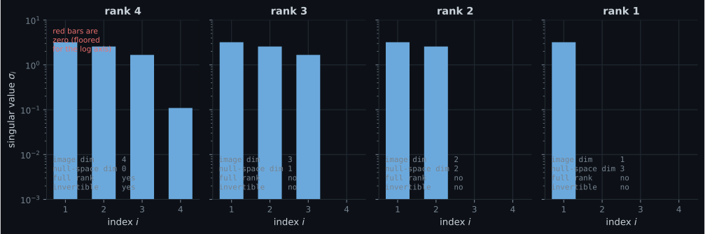
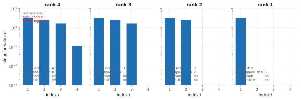
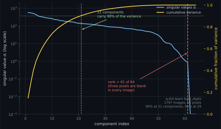
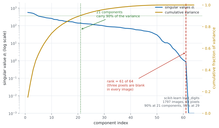
Reading the plot

The second figure is the bridge to Chapter 10, and it makes a point this section’s definitions cannot.

It plots the 8-by-8 handwritten digit images: 1797 of them, 64 pixels each. Two numbers matter.

The rank is 61, not 64. So rank does notice some exact dependence here — and what it noticed is dull: three border pixels are blank in every single image, so three columns are identically zero. That is what exact linear dependence usually looks like in real data. It is a data-collection artefact, not a structural insight.

Twenty-one components carry 90% of the variance, and twenty-nine carry 95%. That redundancy is the interesting kind, and rank is completely blind to it, because those remaining directions are small rather than zero. By the definitions on this page, all 61 surviving directions are equally independent.

So there are two different notions of dimension in play. The algebraic one, rank, is an integer and says 61. The effective one — how many directions matter — is not an integer at all, and depends on how much variance you are willing to discard: 21 at 90%, 29 at 95%.

That gap is the entire opportunity Chapter 10 exploits. PCA does not look for a rank deficiency; it looks for where the spectrum falls off and truncates there. §4.6’s Eckart–Young theorem then says the truncation is the best possible low-rank approximation.

From the book

Mathematics for Machine Learning §2.6.1 gives Definition 2.13 (generating set and span), noting that $\mathcal{A}$ is a generating set if every $\mathbf{v} \in \mathcal{V}$ is a linear combination of its elements, and writing $V = \operatorname{span}[\mathcal{A}]$. Definition 2.14 (basis) defines a generating set as minimal when no smaller subset spans $V$, and states that every linearly independent generating set is minimal and is a basis. The four equivalent characterisations follow — basis, minimal generating set, maximal linearly independent set, and unique representation (Equation 2.77) — with the marginal note that “a basis is a minimal generating set and a maximal linearly independent set of vectors”. Example 2.16 gives the canonical/standard basis of $\mathbb{R}^3$ (Equation 2.78), two other bases (Equation 2.79), and a set that is independent but not a generating set of $\mathbb{R}^4$ (Equation 2.80). The following remarks state that every vector space possesses a basis, that there is no unique basis but all bases have the same number of elements — the dimension $\dim(V)$ — and that $\dim(U) \le \dim(V)$ for a subspace with equality iff $U = V$. A further remark warns that “the dimension of a vector space is not necessarily the number of elements in a vector”, giving $V = \operatorname{span}\!\left[\begin{bmatrix}0\\1\end{bmatrix}\right]$ as a one-dimensional example. The three-step recipe for a basis of a subspace — spanning vectors as columns, row-echelon form, pivot columns — precedes Example 2.17, which finds $\{\mathbf{x}_1,\mathbf{x}_2,\mathbf{x}_4\}$ a basis of a subspace of $\mathbb{R}^5$ (Equations 2.81–2.83). §2.6.2 defines the rank as the common number of linearly independent columns and rows, and its Remark lists the properties used above: $\operatorname{rk}(\mathbf{A}) = \operatorname{rk}(\mathbf{A}^\top)$; the columns span the image or range of dimension $\operatorname{rk}(\mathbf{A})$; the rows span a subspace of the same dimension; $\mathbf{A} \in \mathbb{R}^{n\times n}$ is regular iff $\operatorname{rk}(\mathbf{A}) = n$; $\mathbf{A}\mathbf{x} = \mathbf{b}$ is solvable iff $\operatorname{rk}(\mathbf{A}) = \operatorname{rk}(\mathbf{A}\mid\mathbf{b})$; the solution space of $\mathbf{A}\mathbf{x} = \mathbf{0}$ has dimension $n - \operatorname{rk}(\mathbf{A})$, later called the kernel or null space; and full rank versus rank deficient. Example 2.18 computes two ranks, including via Gaussian elimination (Equation 2.84).

Pitfalls

Dimension counts directions, not components

A line in $\mathbb{R}^{1000}$ is one-dimensional. The book flags this explicitly. Confusing the two is what makes “high-dimensional data” sound hopeless when the data may occupy a very low-dimensional subspace — the observation Chapter 10 is built on.

A basis is not unique; the dimension is

Any two people will produce different bases and the same count. So “the basis” is wrong phrasing unless a specific one has been fixed — and §2.7’s transformation matrices depend on which one, which is why the book insists on ordered bases there.

Spanning and independence are different failures

Too few vectors and you do not span, so some points have no coordinates. Too many and you span but lose uniqueness, so some points have many. A basis is the unique size where neither happens, and the two failure modes are not symmetric — one loses reachability, the other loses well-definedness.

Rank does not detect near-dependence

Two features that are 99.99% collinear give full rank and a catastrophic condition number. Rank is an integer answer to “exactly zero?”; the practical question is “how small?”, answered by the singular values or np.linalg.cond. Every regularisation technique in Chapter 9 exists because rank is the wrong diagnostic here.

Full rank does not mean invertible

Full rank means $\operatorname{rk} = \min(m,n)$. A $2\times4$ matrix of rank 2 has full rank and no inverse, because it is not square. Invertibility needs square and $\operatorname{rk} = n$.

Compare

concept	question it answers	is it unique?
span	what can these vectors reach?	yes — a specific subspace
generating set	do they reach everything?	no — many exist, of many sizes
basis	the smallest set that reaches everything	no — many bases exist
dimension	how many vectors does any basis have?	yes
rank	how many independent directions does a matrix carry?	yes
condition number	how close to dependent are they?	yes, and it is the practical question

pch.quizTag Check yourself

1. Which of these is NOT one of the four equivalent characterisations of a basis?

   A A minimal generating set B A maximal linearly independent set C A set in which every vector has a unique representation D A set whose vectors are mutually orthogonal
   pch.quizShowAnswer

   D — A set whose vectors are mutually orthogonal — Orthogonality is a much stronger extra condition — it makes an ORTHONORMAL basis, which is section 3.5's subject and genuinely more convenient. Plenty of perfectly good bases are not orthogonal.

2. The span of a single two-component vector is what dimension?

   A Two, because the vector has two components B One C Zero D It depends on the vector
   pch.quizShowAnswer

   B — One — Dimension counts independent directions, not entries. The book gives exactly this example as a warning. A line in a thousand-dimensional space is still one-dimensional.

3. A matrix is two-by-four with rank 2. What is the dimension of its null space?

   A Zero B Two C Three D Four
   pch.quizShowAnswer

   B — Two — The null-space dimension is n minus the rank, where n is the number of columns. Four minus two is two. Note this matrix also has full rank, since the maximum possible for its shape is two — and it still has no inverse.

4. Two features in a dataset are 99.99 percent collinear. What does the rank tell you?

   A The rank drops by one, flagging the problem B Nothing useful — the rank is still full, because the dependence is not exact. The condition number is the diagnostic C The rank becomes non-integer D The matrix becomes singular
   pch.quizShowAnswer

   B — Nothing useful — the rank is still full, because the dependence is not exact. The condition number is the diagnostic — Rank answers 'exactly zero?' and the answer is no. Near dependence shows up as a tiny singular value and a huge condition number, which is why regularisation exists rather than a rank check.

🧪 Try It Yourself

Exercise 1 – Extract a basis from a spanning set

pch.exerciseTag pch.exerciseTitle

Exercise 2 – Row rank equals column rank

pch.exerciseTag pch.exerciseTitle

Exercise 3 – The null-space dimension

pch.exerciseTag pch.exerciseTitle

Exercise 4 – Uniqueness is what minimality buys

pch.exerciseTag pch.exerciseTitle

Exercise 5 – Rank is blind to near-dependence

pch.exerciseTag pch.exerciseTitle

Recall card

• The span of a set is every linear combination of it, and a span is always a subspace — which is how subspaces are manufactured.
• A generating set reaches everything; a basis is a generating set that is also minimal, equivalently linearly independent.
• Four equivalent characterisations of a basis — basis, minimal generating set, maximal independent set, and unique representation of every vector.
• A basis is squeezed from both sides: minimal among spanning sets and maximal among independent sets simultaneously.
• Uniqueness of coordinates IS linear independence rewritten — subtract two representations and independence forces the difference to vanish.
• No basis is unique but every basis of a space has the same size, and that invariant number is the dimension.
• Dimension counts independent directions, not components — a line in a thousand-dimensional space is one-dimensional.
• A basis of a subspace comes from three steps: spanning vectors as columns, row-echelon form, keep the pivot columns.
• Row rank equals column rank, always — two counts about vectors in different spaces that never disagree.
• Rank decides invertibility, solvability, image dimension and null-space dimension — the null space has dimension $n$ minus the rank.
• Full rank is not the same as invertible: full rank means the most its shape allows, and a non-square matrix can never be inverted.
• Rank is blind to near-dependence. It answers “exactly zero?”; the practical question is “how small?”, answered by the singular values and the condition number.

Next: functions that are secretly matrices — Linear Mappings.