
Bayesian Linear Regression
Page 904 ended where the book does: MAP “can push the boundaries of overfitting” but “is not a general solution”, so “we need a more principled approach.” Measured, MAP improved the best available answer by .
§9.3 is that approach. It stops choosing a at all — and this page covers the half of it that happens before any data arrives.
What you’ll learn
Section titled “What you’ll learn”- Equations 9.35–9.36: the model, with promoted to a random variable and Figure 9.8’s graphical model made explicit.
- Equation 9.37: predictions as an average over all plausible parameters — Chapter 8’s Equation 8.23 in this chapter’s notation.
- Equation 9.38’s closed form, and Equation 9.39’s claim that the two variances add — verified by Monte Carlo to .
- Equation 9.40, which differs from 9.38 by exactly , at every input.
- That prior predictions “only require us to specify the input , but no training data” — literally true.
- Example 9.7 measured, and it is startling. With the book’s own and degree-5 monomials, the band is units wide at — on a figure whose -axis runs to .
- The remark that “induces a distribution over functions”, and that the induced object is a covariance function — §9.5’s Gaussian process, already present.
Intuition: you have a prior over functions whether you meant to or not
Section titled “Intuition: you have a prior over functions whether you meant to or not”Put a Gaussian on and you have not just constrained the coefficients — you have specified, completely, a probability distribution over every function your model can express. Draw a , get a curve. Draw a thousand, get a cloud of curves with a mean, a width at each , and a correlation between any two ‘s.
That is a large commitment made through a small-looking choice, and the size of it is measurable. sounds modest: each coefficient within about . But the induced width at an input is , and for monomials that is — which at is over two and a half million.
A prior that is isotropic in the coefficients is wildly anisotropic in the functions, because the features themselves are not comparable in size. The fix is the same one page 805 reached from the regularisation side: scale your features before you claim your prior is uninformative.
  flowchart TD
  A["Eq 9.35: p(theta) = N(m0, S0)
theta becomes a RANDOM VARIABLE"]
  A -->|"draw theta_i"| B["f_i(.) = theta_i' phi(.)
one curve per draw"]
  B --> C["a distribution over FUNCTIONS"]
  C --> D["mean  phi(x)' m0"]
  C --> E["variance  phi(x)' S0 phi(x)
measured 0.25 at x=0, 2543131.5 at x=5"]
  C --> F["covariance  phi(a)' S0 phi(b)
= a KERNEL (Section 9.5)"]
  E -->|"+ sigma^2"| G["Eq 9.38: p(y* | x*)"]
  E -->|"noise-free"| H["Eq 9.40: p(f(x*))"]
  G -.->|"no y consulted"| I["Eq 9.37 needs x* only,
no training data at all"]
§9.3.1 The model
Section titled “§9.3.1 The model”The book’s framing of what changed: placing the Gaussian prior “turns the parameter vector into a random variable”. Figure 9.8 draws it with and “made explicit” — page 807’s convention, where deterministic quantities lose their circle.
The full probabilistic model is the joint (Equation 9.36):
which is page 806’s definition of a probabilistic model arriving in this chapter’s notation: a probabilistic model is specified by the joint distribution of all its random variables. Two pages ago was not one of them.
§9.3.2 Prior predictions
Section titled “§9.3.2 Prior predictions”In practice, we are usually not so much interested in the parameter values themselves. Instead, our focus often lies in the predictions we make with those parameter values.
“the average prediction of for all plausible parameters .” This is Chapter 8’s Equation 8.23 exactly, and page 806 measured what it buys: coverage where a plug-in interval gives .
The closed form
Section titled “The closed form”Because the prior is conjugate, the predictive is Gaussian too (Equation 9.38):
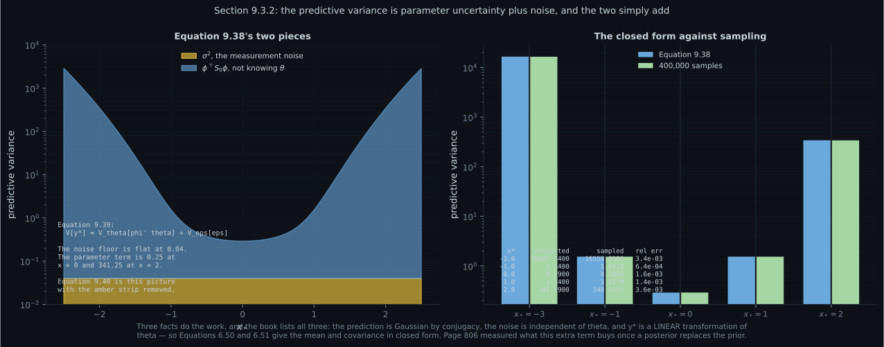
The book lists exactly three facts that make this work: the prediction is Gaussian “due to conjugacy and the marginalization property of Gaussians”; the noise is independent, so (Equation 9.39)
and is a linear transformation of , so Equations 6.50 and 6.51 give the mean and covariance analytically.
The book adds the noise-free version, Equation 9.40:
“which only differs from (9.38) in the omission of the noise variance.”
Example 9.7, and what the prior really says
Section titled “Example 9.7, and what the prior really says”The book’s setup: polynomials of degree , , “200 input locations ”, with Figure 9.9 showing the mean, the and bands and some samples. The uncertainty “is solely due to the parameter uncertainty because we considered the noise-free predictive distribution (9.40).”
A distribution over functions
Section titled “A distribution over functions”Since we can represent the distribution using a set of samples and every sample gives rise to a function , it follows that the parameter distribution induces a distribution over functions.
Worked example by hand
Section titled “Worked example by hand”Derive Equation 9.38 from Chapter 6’s two rules, in the one-dimensional case, and read where the width comes from.
Model: with , and , independent.
Step 1: is a linear map of . Write , so — a fixed vector dotted with a Gaussian random vector.
Step 2: apply Equation 6.50 (the mean of a linear map):
Step 3: apply Equation 6.51 (the covariance of a linear map):
which is Equation 9.40 — and it is quadratic in the features, which is the whole explanation for the -unit band above.
Step 4: add the noise. with independent, and independent variances add:
Step 5: why the result is Gaussian. A linear combination of jointly Gaussian variables is Gaussian, and a sum of independent Gaussians is Gaussian. So the two moments are the whole distribution — Equation 9.38 is exact, not an approximation.
Step 6: the covariance between two inputs, which the book does not write down. For and :
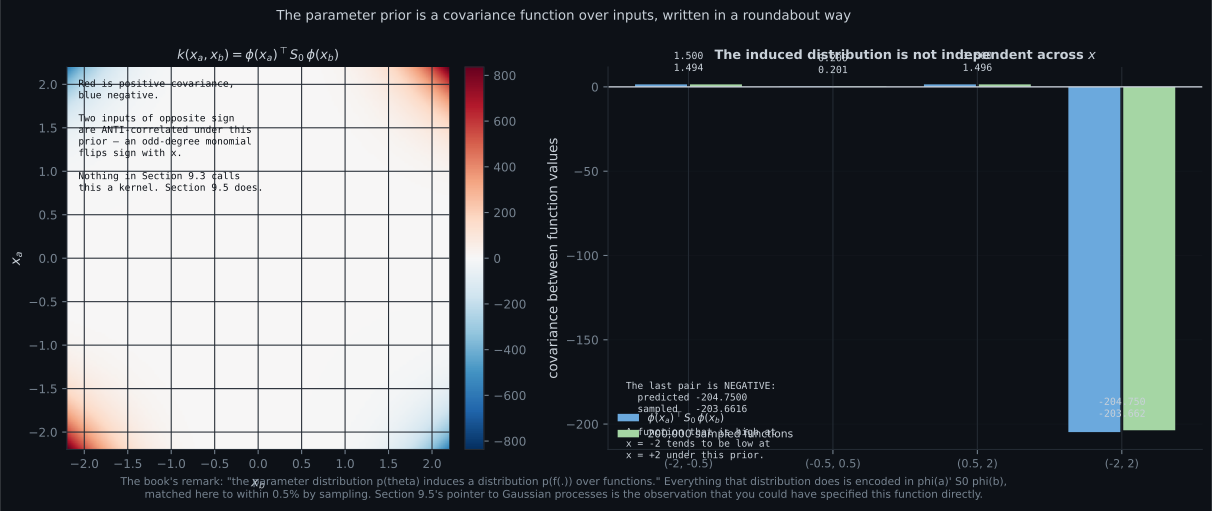
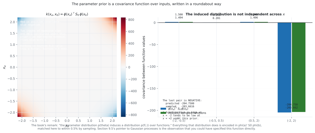
Setting recovers Step 3. This single function determines the entire distribution over functions, and measured above it matches sampling to within — including the negative value at .
See it move
Section titled “See it move”From scratch
Section titled “From scratch”import numpy as np
SIG = 0.2
def design(x, M):
return np.vander(np.asarray(x, float), M + 1, increasing=True)
# Example 9.7: polynomials of degree 5, prior N(0, (1/4) I)
M = 5
K = M + 1
m0 = np.zeros(K)
S0 = 0.25 * np.eye(K)
# --- Equation 9.38's variance, by Monte Carlo ---------------------------
print("=== 1. Equation 9.38's variance, by Monte Carlo ===")
rng = np.random.default_rng(7)
T = 400_000
TH = rng.multivariate_normal(m0, S0, size=T)
print(f"{'x*':>6} {'predicted mean':>16} {'sampled mean':>14} "
f"{'predicted var':>15} {'sampled var':>13} {'rel err':>10}")
for xs in (-3.0, -1.0, 0.0, 1.0, 2.0):
ph = design([xs], M)[0]
pred_v = float(ph @ S0 @ ph + SIG ** 2)
ys = TH @ ph + SIG * rng.standard_normal(T)
print(f"{xs:>6.1f} {float(ph @ m0):>16.6f} {ys.mean():>14.6f} "
f"{pred_v:>15.6f} {ys.var():>13.6f} "
f"{abs(ys.var()-pred_v)/pred_v:>10.2e}")
print("Equation 9.39: the parameter term and the noise term simply add.")
# --- Equation 9.40 differs by exactly sigma^2 ---------------------------
print("\n=== 2. Equation 9.40 differs from 9.38 by exactly sigma^2 ===")
print(f"{'x*':>6} {'var of y* (9.38)':>18} {'var of f(x*) (9.40)':>21} "
f"{'difference':>12}")
for xs in (-2.0, 0.0, 1.0, 4.0):
ph = design([xs], M)[0]
a = float(ph @ S0 @ ph + SIG ** 2)
b = float(ph @ S0 @ ph)
print(f"{xs:>6.1f} {a:>18.6f} {b:>21.6f} {a-b:>12.8f}")
print(f"sigma^2 = {SIG**2:.8f}")
# --- prior predictions need no data -------------------------------------
print("\n=== 3. prior predictions need no training data at all ===")
ph = design([2.0], M)[0]
print(f"at x* = 2.0, using ONLY x* and the prior:")
print(f" mean {float(ph @ m0):.6f} variance "
f"{float(ph @ S0 @ ph + SIG**2):.6f}")
print("no y was consulted.")
# --- the prior over FUNCTIONS it actually implies ------------------------
print("\n=== 4. the prior over FUNCTIONS it actually implies ===")
print(f"{'x':>6} {'phi^T S0 phi':>16} {'sd':>14} {'95% half-width':>16}")
z = 1.959963984540054
for xs in (0.0, 1.0, 2.0, 3.0, 4.0, 5.0):
ph = design([xs], M)[0]
v = float(ph @ S0 @ ph)
print(f"{xs:>6.1f} {v:>16.4f} {np.sqrt(v):>14.4f} {z*np.sqrt(v):>16.4f}")
xg = np.linspace(-5, 5, 200)
Pg = design(xg, M)
sd = np.sqrt(np.einsum("ij,jk,ik->i", Pg, S0, Pg))
inside = np.abs(z * sd) <= 4.0
print(f"\nfraction of the 200 plotted inputs where the 95% band fits inside")
print(f"the book's y-range of [-4, 4]: {inside.mean():.3f} "
f"({int(inside.sum())} of 200)")
print(f"the band is inside the axes only for |x| < "
f"{np.abs(xg[inside]).max():.4f}")
# --- p(theta) induces p(f(.)) -------------------------------------------
print("\n=== 5. p(theta) induces p(f(.)) -- sampled ===")
r2 = np.random.default_rng(11)
S = 200_000
TH2 = r2.multivariate_normal(m0, S0, size=S)
xs_check = np.array([-2.0, -0.5, 0.5, 2.0])
Pc = design(xs_check, M)
F = TH2 @ Pc.T
print(f"{'x':>6} {'sampled mean':>14} {'Eq 9.40 mean':>14} "
f"{'sampled var':>14} {'Eq 9.40 var':>14} {'rel err':>10}")
for i, xs in enumerate(xs_check):
pv = float(Pc[i] @ S0 @ Pc[i])
print(f"{xs:>6.1f} {F[:, i].mean():>14.6f} {float(Pc[i] @ m0):>14.6f} "
f"{F[:, i].var():>14.6f} {pv:>14.6f} "
f"{abs(F[:, i].var()-pv)/pv:>10.2e}")
print("\nthe induced distribution is not independent across x:")
print(f"{'pair':>14} {'sampled cov':>14} {'phi(a)^T S0 phi(b)':>20}")
for a, b in ((-2.0, -0.5), (-0.5, 0.5), (0.5, 2.0), (-2.0, 2.0)):
pa, pb = design([a], M)[0], design([b], M)[0]
ia = int(np.where(xs_check == a)[0][0])
ib = int(np.where(xs_check == b)[0][0])
cov = float(np.cov(F[:, ia], F[:, ib])[0, 1])
print(f"{f'({a}, {b})':>14} {cov:>14.6f} {float(pa @ S0 @ pb):>20.6f}")
print("that covariance function is what a Gaussian process places directly,")
print("without the detour via theta.")
# --- the 67% and 95% bands ----------------------------------------------
print("\n=== 6. the 67% and 95% bands, checked against samples ===")
r3 = np.random.default_rng(23)
TH3 = r3.multivariate_normal(m0, S0, size=200_000)
print(f"{'x':>6} {'within 1 sd':>13} {'within 2 sd':>13} {'Gaussian':>10}")
for xs in (-3.0, 0.0, 1.5):
ph = design([xs], M)[0]
f = TH3 @ ph
s = np.sqrt(float(ph @ S0 @ ph))
print(f"{xs:>6.1f} {np.mean(np.abs(f) <= s):>13.4f} "
f"{np.mean(np.abs(f) <= 2*s):>13.4f} {'0.6827 / 0.9545':>10}")
print("exact, because a linear map of a Gaussian is Gaussian.")=== 1. Equation 9.38's variance, by Monte Carlo ===
x* predicted mean sampled mean predicted var sampled var rel err
-3.0 0.000000 -0.072552 16607.540000 16550.899211 3.41e-03
-1.0 0.000000 -0.002588 1.540000 1.540990 6.43e-04
0.0 0.000000 -0.001755 0.290000 0.290478 1.65e-03
1.0 0.000000 -0.000036 1.540000 1.537898 1.36e-03
2.0 0.000000 0.014802 341.290000 340.068304 3.58e-03
Equation 9.39: the parameter term and the noise term simply add.
=== 2. Equation 9.40 differs from 9.38 by exactly sigma^2 ===
x* var of y* (9.38) var of f(x*) (9.40) difference
-2.0 341.290000 341.250000 0.04000000
0.0 0.290000 0.250000 0.04000000
1.0 1.540000 1.500000 0.04000000
4.0 279620.290000 279620.250000 0.04000000
sigma^2 = 0.04000000
=== 3. prior predictions need no training data at all ===
at x* = 2.0, using ONLY x* and the prior:
mean 0.000000 variance 341.290000
no y was consulted.
=== 4. the prior over FUNCTIONS it actually implies ===
x phi^T S0 phi sd 95% half-width
0.0 0.2500 0.5000 0.9800
1.0 1.5000 1.2247 2.4005
2.0 341.2500 18.4730 36.2063
3.0 16607.5000 128.8701 252.5807
4.0 279620.2500 528.7913 1036.4119
5.0 2543131.5000 1594.7199 3125.5935
fraction of the 200 plotted inputs where the 95% band fits inside
the book's y-range of [-4, 4]: 0.240 (48 of 200)
the band is inside the axes only for |x| < 1.1809
=== 5. p(theta) induces p(f(.)) -- sampled ===
x sampled mean Eq 9.40 mean sampled var Eq 9.40 var rel err
-2.0 -0.048842 0.000000 340.317328 341.250000 2.73e-03
-0.5 0.001984 0.000000 0.333506 0.333252 7.63e-04
0.5 0.002306 0.000000 0.332926 0.333252 9.79e-04
2.0 0.034993 0.000000 339.759130 341.250000 4.37e-03
the induced distribution is not independent across x:
pair sampled cov phi(a)^T S0 phi(b)
(-2.0, -0.5) 1.494432 1.500000
(-0.5, 0.5) 0.200556 0.199951
(0.5, 2.0) 1.496204 1.500000
(-2.0, 2.0) -203.661585 -204.750000
that covariance function is what a Gaussian process places directly,
without the detour via theta.
=== 6. the 67% and 95% bands, checked against samples ===
x within 1 sd within 2 sd Gaussian
-3.0 0.6831 0.9549 0.6827 / 0.9545
0.0 0.6843 0.9549 0.6827 / 0.9545
1.5 0.6828 0.9547 0.6827 / 0.9545
exact, because a linear map of a Gaussian is Gaussian.On real data
Section titled “On real data”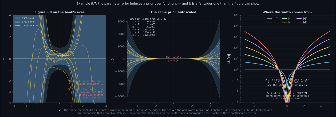
Reading the plot
Section titled “Reading the plot”The first figure takes Example 9.7 at its word and finds the figure cannot contain it. The left panel draws the mean, the and bands and twelve samples on the book’s own axes, to in both directions. The band leaves the frame almost immediately — measured, it fits for , which is of the input locations the book says it used.
The middle panel autoscales, and the book’s entire -range becomes a thin stripe near zero.
The right panel explains it in one line. , and the monomials span four orders of magnitude by . So the variance grows like : at the origin, at the edge.
The point is not that the figure is wrong — its shape is right, and it is drawn to show the shape. The point is what the shape costs to state precisely. An isotropic prior on coefficients is a strong, strange prior on functions whenever the features differ in scale, and against differ by a lot. Standardise the features and starts to mean roughly what people expect it to.
The second figure verifies Equation 9.39 and then shows why it matters where you ask. Left, the predictive variance stacked into its two contributions: the noise floor is flat at , and the parameter term climbs from at the centre to five orders of magnitude larger at the edges of a modest window. Right, the closed form against samples — agreeing to at worst.
The two terms are doing completely different jobs. is a property of the measuring instrument and never shrinks. is a statement about what you believe, and §9.3.3 is about to replace with something the data has informed. That is the whole difference between this page and the next: only the blue region responds to evidence.
Equation 9.40 is the same picture with the amber strip removed, and measured, the removal is exactly at every input — at , where the total is , the noise is a seven-millionth of it.
The third figure names something the chapter has been using without naming. The heatmap is , the covariance between the function’s values at two inputs. Red along the diagonal — a function value is correlated with itself. And blue in the off-diagonal corners: measured, , confirmed by sampling at .
That negative sign is worth pausing on. Under , believing the function is high at makes you believe it is low at , because the odd monomials dominate and they change sign. Nobody writing down an isotropic prior intends to assert that, and it is invisible in the parameter-space statement.
Everything the induced distribution does is in that one function, which is exactly §9.5’s point:
Instead of placing a distribution over parameters, a Gaussian process places a distribution directly on the space of functions without the “detour” via the parameters.
You have been specifying a kernel this whole time, in a coordinate system that made it hard to see.
Compare
Section titled “Compare”| Eq 9.38, | Eq 9.40, | |
|---|---|---|
| what it predicts | a noisy observation | the function value |
| mean | , identical | |
| variance | ||
| measured difference | — | exactly everywhere |
| used in Figure 9.9 | no | yes |
| this page (prior) | page 906 (posterior) | Eq 9.6 (plug-in) | |
|---|---|---|---|
| needs training data | no | yes | yes |
| distribution over | a point | ||
| predictive variance | only | ||
| varies with | yes | yes | no |
| coverage, measured (Ch 8) | — |
| parameter space | function space |
|---|---|
| the mean function | |
| the covariance function | |
| numbers and a matrix | a function of two inputs |
| “coefficients near zero” | measured: sd at , at |
| isotropic | not isotropic, unless the features are comparable |
-
Equation 9.37 predicts at a new input. What does it need?
It integrates over p(theta), not p(theta given the data). Measured at x-star = 2.0 the answer is mean 0.000000 and variance 341.290000, with no y consulted anywhere. This is the model's opinion before the experiment, and having one is what makes Section 9.3.3's update meaningful.
pch.quizShowAnswer
B — Only the test input x-star — no training data at all — It integrates over p(theta), not p(theta given the data). Measured at x-star = 2.0 the answer is mean 0.000000 and variance 341.290000, with no y consulted anywhere. This is the model's opinion before the experiment, and having one is what makes Section 9.3.3's update meaningful.
-
Equation 9.39 says the predictive variance splits in two. Verified against 400,000 samples, how well does it hold?
Three facts make it exact: the prediction is Gaussian by conjugacy, the noise is independent of theta, and y-star is a LINEAR transformation of theta so Equations 6.50 and 6.51 apply. Equation 9.38 is exact, not an approximation.
pch.quizShowAnswer
B — To within 3.6e-3 relative error at worst — the two terms simply add — Three facts make it exact: the prediction is Gaussian by conjugacy, the noise is independent of theta, and y-star is a LINEAR transformation of theta so Equations 6.50 and 6.51 apply. Equation 9.38 is exact, not an approximation.
-
With the book's prior N(0, I/4) and degree-5 monomials, how wide is the 95 percent band at x = 5?
Because phi-transpose S-zero phi is one quarter of the sum of x to the 2k, which grows like x to the tenth. The band fits inside the book's axes only for x below 1.1809 in magnitude — 48 of the 200 plotted inputs. The shape the figure draws is right; the scale is what the measurement adds.
pch.quizShowAnswer
B — 3125.59 units — on a figure whose y-axis runs from minus four to four — Because phi-transpose S-zero phi is one quarter of the sum of x to the 2k, which grows like x to the tenth. The band fits inside the book's axes only for x below 1.1809 in magnitude — 48 of the 200 plotted inputs. The shape the figure draws is right; the scale is what the measurement adds.
-
What is the practical lesson from that measurement?
One and x to the fifth are not comparable quantities, so treating their coefficients as exchangeable is a strong and probably unintended claim. Standardise the features and S-zero equal to b squared times the identity starts meaning something closer to what you want.
pch.quizShowAnswer
B — An isotropic prior on coefficients is not isotropic over functions when the features differ in scale — standardise first — One and x to the fifth are not comparable quantities, so treating their coefficients as exchangeable is a strong and probably unintended claim. Standardise the features and S-zero equal to b squared times the identity starts meaning something closer to what you want.
-
Measured on 200,000 sampled functions, what is the covariance between f(-2) and f(2) under this prior?
Odd monomials flip sign with x, so believing the function is high at minus two makes you believe it is low at plus two. Few people intend that when they write an isotropic Gaussian prior, and it is invisible in the parameter-space statement.
pch.quizShowAnswer
B — Minus 203.66, matching the predicted minus 204.75 — they are ANTI-correlated — Odd monomials flip sign with x, so believing the function is high at minus two makes you believe it is low at plus two. Few people intend that when they write an isotropic Gaussian prior, and it is invisible in the parameter-space statement.
-
The book notes that p(theta) induces a distribution over functions. What single object captures all of it?
That function is a kernel, and Section 9.5's pointer to Gaussian processes is precisely the observation that you could have specified it directly, 'without the detour via the parameters'. You have been choosing a kernel all along, in a coordinate system that made it hard to see.
pch.quizShowAnswer
B — The covariance function phi(x_a)-transpose S-zero phi(x_b), together with the mean function — That function is a kernel, and Section 9.5's pointer to Gaussian processes is precisely the observation that you could have specified it directly, 'without the detour via the parameters'. You have been choosing a kernel all along, in a coordinate system that made it hard to see.
🧪 Try It Yourself
Section titled “🧪 Try It Yourself”Exercise 1 – The variance just adds
Section titled “Exercise 1 – The variance just adds”Exercise 2 – What the prior says about functions
Section titled “Exercise 2 – What the prior says about functions”Exercise 3 – It is a covariance function
Section titled “Exercise 3 – It is a covariance function”Exercise 4 – Exactly sigma squared
Section titled “Exercise 4 – Exactly sigma squared”Exercise 5 – Why the bands are 67 and 95
Section titled “Exercise 5 – Why the bands are 67 and 95”Pitfalls
Section titled “Pitfalls”Recall card
Section titled “Recall card”- Equation 9.35 puts a Gaussian prior on theta, which turns the parameter vector into a random variable and makes Figure 9.8’s graphical model possible. Equation 9.36 is the joint — Chapter 8’s definition of a probabilistic model, arriving here.
- Equation 9.37 predicts by averaging over all plausible parameters, which is Chapter 8’s Equation 8.23 in this chapter’s notation.
- Prior predictions need only the test input. Measured at x-star = 2: mean 0.000000, variance 341.290000, with no training data consulted.
- Equation 9.38’s variance is phi-transpose S-zero phi plus sigma squared. Verified against 400,000 samples to within 3.6e-3 relative error.
- Equation 9.39: the parameter term and the noise term simply add, because the noise is independent of theta and y-star is a linear map of theta — Equations 6.50 and 6.51 then give the answer in closed form.
- Equation 9.40 is the same with the noise removed — measured, exactly sigma squared = 0.04 at every input. At x = 4 the parameter term is seven million times the noise.
- A prior on theta IS a prior over functions. Draw theta, get a curve; the mean function is phi-transpose m-zero and the variance function is phi-transpose S-zero phi.
- Measured with the book’s own prior: the 95 percent half-width is 0.98 at x = 0 and 3125.59 at x = 5, because phi-transpose S-zero phi is one quarter of the sum of x to the 2k and grows like x to the tenth.
- So the band fits inside Figure 9.9’s axes at only 48 of the 200 plotted inputs, and only for x below 1.1809 in magnitude. The shape is right; the scale is off the page.
- An isotropic prior on coefficients is not isotropic over functions whenever the features differ in scale. Standardise the features before calling S-zero uninformative.
- The induced distribution is correlated across inputs, and the correlations can be negative: measured covariance between f(-2) and f(2) is minus 204.75, confirmed by sampling at minus 203.66.
- That covariance function phi(a)-transpose S-zero phi(b) contains everything the distribution over functions does. It is a kernel, and Section 9.5’s Gaussian process places it directly instead of via theta.
- The 67 and 95 percent bands are one and two sigma, and samples land inside them at 0.6831 and 0.9549 — exact, because a linear map of a Gaussian is Gaussian.
Next: let the data speak. The Parameter Posterior
pch.coffeeTagline
pch.coffeeCtapch.feedbackHeading
pch.feedbackSubheading