
Time Series Forecasting Fundamentals
What you’ll learn
Section titled “What you’ll learn”- why every baseline comparison must be against naive and seasonal naive, and what MASE is
- the measured cost of a shuffled split: MAE 6.72 reported against 10.41 honest
- how to build lag features that cannot see their own target
- the leak that looks like a 25% win: 6.852 → 5.147 MAE from
rolling(7, center=True) - one-step against multi-step error: 3.73 at horizon 1 and 9.03 at horizon 28
- why is close to meaningless on a trending series
The series
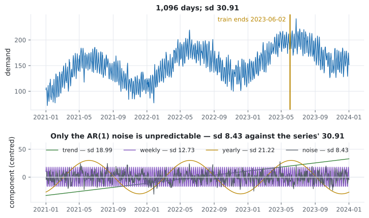
Section titled “The series”Three years of daily demand, built from four known components so that we can say exactly how much of it any model is entitled to explain.
rng = np.random.default_rng(4)
t = np.arange(1096)

trend = 120 + 0.06 * t
weekly = 18 * np.sin(2 * np.pi * (t % 7) / 7 + 0.6)
yearly = 30 * np.sin(2 * np.pi * t / 365.25 - 1.1)

noise = np.zeros(1096)                      # AR(1): today's error remembers yesterday
for i in range(1, 1096):
    noise[i] = 0.55 * noise[i - 1] + rng.normal(0, 7)

y = pd.Series(trend + weekly + yearly + noise,
              index=pd.date_range("2021-01-01", periods=1096, freq="D"))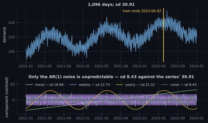
| Component | Standard deviation |
|---|---|
| trend | 18.99 |
| weekly season | 12.73 |
| yearly season | 21.22 |
| AR(1) noise | 8.43 |
| the series | 30.91 |
Those standard deviations do not combine into a tidy variance decomposition — trend and yearly season are correlated over a three-year window, so the shares would sum to more than 100%. The number that matters is the last one against the second-to-last: about 8.4 of the series’ 30.9 of variation is noise, and even that is autocorrelated.
The AR(1) structure sets the floor. With innovations of standard deviation 7, a perfect one-step forecast still has MAE . No model on this page can beat that, and any model that appears to has seen the future.
Baselines first, always
Section titled “Baselines first, always”Two forecasts require no model at all:
- naive: tomorrow equals today,
- seasonal naive: tomorrow equals the same weekday last week,
On a chronological 80/20 split — 854 training days, then 214 test days from 2023-06-02:
| Forecast | MAE | MASE | |
|---|---|---|---|
| naive (yesterday) | 12.174 | 0.6371 | 1.000 |
| seasonal naive (last week) | 10.474 | 0.7219 | 0.860 |
| the training mean | 30.200 | −1.2496 | 2.481 |
MASE — mean absolute scaled error — is MAE divided by the naive forecast’s MAE. Below 1 means you beat “tomorrow is like today”; above 1 means you did not. It is the honest headline for a forecasting model because it is scale-free and it has a meaningful zero point.
Note the training mean’s of −1.2496. On a trending series the test window’s mean is nowhere near the training window’s, so predicting the training mean is worse than useless — and , which compares against the test window’s own mean, hides how bad a forecast is while flattering anything that tracks the level. Report MAE and MASE. Use only if someone insists.
A model on lag features
Section titled “A model on lag features”The standard move is to turn the series into a supervised table, where every column is a shifted copy of the past:
def lag_frame(series, lags=(1, 2, 3, 7, 14), roll=(7, 28)):
    """Every column is shifted before use, so no row can see its own target."""
    df = pd.DataFrame({"y": series})
    for L in lags:
        df[f"lag_{L}"] = series.shift(L)
    for w in roll:
        df[f"roll_{w}"] = series.shift(1).rolling(w).mean()   # shift, THEN roll
    df["dow"] = series.index.dayofweek
    df["t"] = np.arange(len(series))
    return df.dropna()
The shift(1) before .rolling() is the whole trick, and leaving it out is the subject of a later
section. With those nine features:
| Model | MAE | RMSE | MASE | |
|---|---|---|---|---|
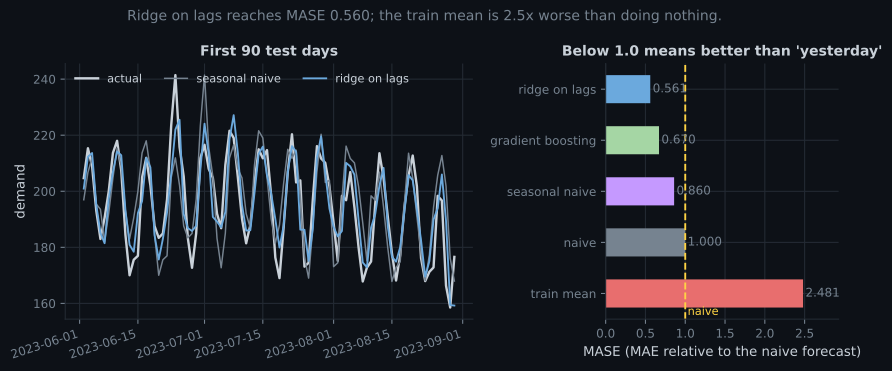
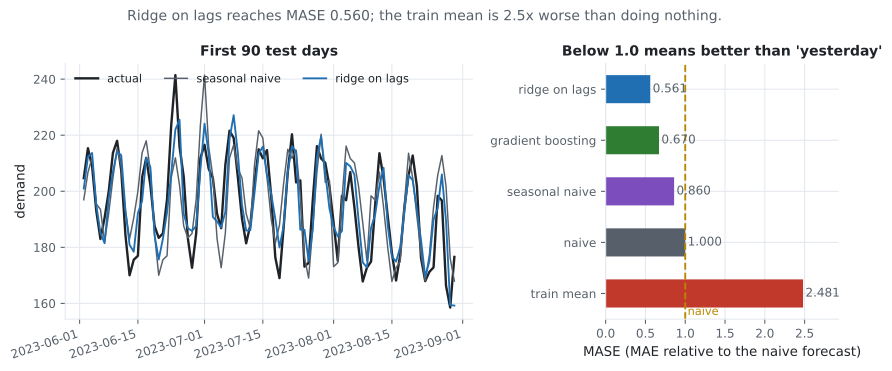
| ridge on lags | 6.824 | 8.491 | 0.8772 | 0.561 |
| gradient boosting | 8.161 | 10.030 | 0.8286 | 0.670 |
| perfect one-step forecast | ≈5.59 | ≈7.00 | ≈0.46 |
Ridge lands at 6.824 against a floor of about 5.59. The remaining gap is mostly the part of the AR(1) noise that a linear function of past values cannot capture, plus estimation error.
Gradient boosting losing to ridge is worth pausing on. Tree ensembles cannot extrapolate: their predictions are averages of training targets, so on a series whose level rises by 0.06 per day they are structurally behind. The usual fix is to model the difference rather than the level, or to detrend first — both of which are decisions about the data, not about the model.
The shuffled split lies, and it lies more to flexible models
Section titled “The shuffled split lies, and it lies more to flexible models”KFold(shuffle=True) puts a Tuesday from 2022 in the training set and the Wednesday next to it in
the test set. The model then interpolates between neighbours that in deployment would not exist.
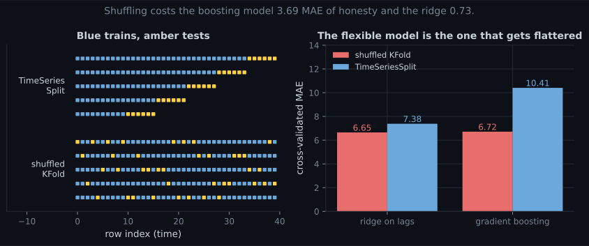
| Model | Shuffled KFold | TimeSeriesSplit | Chronological holdout | Optimism |
|---|---|---|---|---|
| ridge on lags | 6.649 | 7.383 | 6.824 | +0.734 |
| gradient boosting | 6.717 | 10.410 | 8.161 | +3.693 |
Three observations.
The ranking flips. Shuffled cross-validation says the two models are within 0.07 MAE of each other. Time-ordered says the gap is 3.03. Anyone selecting a model on the shuffled number has a 50% chance of shipping the worse one, and no way to know.
Flexible models gain more from leakage. Boosting can memorise local structure that a linear model cannot, so handing it adjacent days is worth 3.69 MAE to it and 0.73 to the ridge. Leakage is not a constant tax; it is a distortion that reorders your candidates.
TimeSeriesSplit is pessimistic on purpose. Its early folds train on as little as one sixth of
the data, so its 7.383 is worse than the 6.824 the model achieves after training on 80%. That is the
right direction to be wrong in: it under-promises and the holdout over-delivers.
The leak that looks like a 25% win
Section titled “The leak that looks like a 25% win”Feature engineering on a series is where leakage becomes invisible, because the offending code looks like every pandas tutorial ever written.
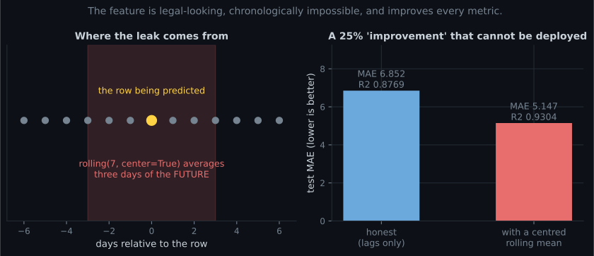
# WRONG: center=True averages rows t-3 .. t+3
frame["roll_centred"] = y.rolling(7, center=True).mean()

# RIGHT: shift first, so the window ends yesterday
frame["roll_7"] = y.shift(1).rolling(7).mean()| Features | Test MAE | Test |
|---|---|---|
| lags and past rolling means only | 6.852 | 0.8769 |
the same plus rolling(7, center=True) | 5.147 | 0.9304 |
The 5.147 is the diagnostic. A perfect one-step forecast on this series has MAE ≈ 5.59, so any number below that is impossible and indicates that information from the future has arrived. Knowing your noise floor is the cheapest leakage detector you will ever build.
Other members of the same family, all of which have shipped to production somewhere:
.rolling(...).mean()without a preceding.shift(1)— includes today’s value in today’s feature.- Group statistics (mean sales per store) computed over the full history, then used to predict the early part of that history.
- Interpolating missing values with
.interpolate()before splitting, which fills gaps using later observations. - Scaling with a
StandardScalerfitted on the whole series, so the test period’s mean influences the training features. - Any feature derived from a column that is itself recorded after the prediction is made — a delivery date, a settled amount, a refund flag.
One step ahead is not a forecast
Section titled “One step ahead is not a forecast”The 6.824 above answers “given everything up to yesterday, what is today?” — which is only useful if you genuinely get yesterday’s value before predicting today. Planning questions are not like that. To forecast 28 days you must feed your own predictions back in as inputs.
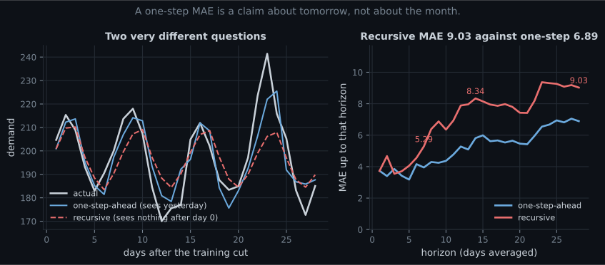
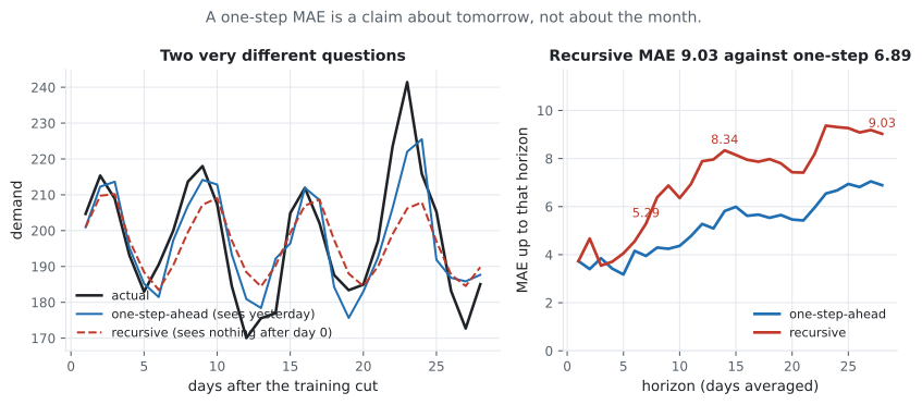
| Horizon | Recursive MAE | One-step MAE |
|---|---|---|
| 1 day | 3.732 | 3.732 |
| 7 days | 5.287 | 3.948 |
| 14 days | 8.340 | 5.815 |
| 28 days | 9.028 | 6.891 |
Two things are happening at once, and only one of them is error accumulation.
Errors compound. Each prediction becomes the next row’s lag_1, so a mistake propagates. For an
AR(1) process with coefficient , the -step-ahead forecast variance grows as
which for saturates at — the variance of the series itself. Beyond about 6 steps the AR(1) part of the forecast has decayed to the unconditional mean and contributes nothing.
The forecast flattens. Feeding predictions back in produces a smoother input series than reality, so the seasonal amplitude shrinks. This is visible in the left panel: the recursive line’s peaks are consistently short of the actual peaks.
The alternatives, both of which sidestep recursion:
- Direct multi-step: fit a separate model per horizon, each predicting from information at . No compounding, models to maintain, and each one gets less relevant features.
- Multi-output: one model, outputs. Shares structure across horizons; supported natively by
linear models and by
MultiOutputRegressor.
Whatever you choose, report the error at the horizon you will actually forecast at. A one-step MAE next to a monthly planning claim is a category error.
See it move
Section titled “See it move”Forecast uncertainty for an AR(1) process is exactly computable, so the decay of a recursive forecast can be watched rather than argued about. Drag — the memory of the process — and see how far into the future the forecast is worth anything.
At the signal is gone after 4 steps: a recursive forecast beyond that point is predicting the seasonal pattern and the trend, and nothing else. At it survives 45 steps, which is why highly persistent series (stock levels, temperatures, populations) forecast much further than mean-reverting ones (returns, click rates) even when both look equally noisy.
The workflow
Section titled “The workflow” flowchart TD
A["An ordered series"] --> B["Plot it. Find the trend,
the seasonality, the gaps"]
B --> C["Compute naive and
seasonal naive MAE"]
C --> D["Build lag features —
shift BEFORE rolling"]
D --> E["TimeSeriesSplit
never shuffle"]
E --> F{"MASE below 1?"}
F -->|"no"| G["Ship the seasonal naive.
Seriously."]
F -->|"yes"| H{"What horizon does
the decision need?"}
H -->|"one step"| I["Report one-step MAE
and MASE"]
H -->|"many steps"| J["Recursive, direct or
multi-output — then report
error AT that horizon"]
I --> K["Check: is the error below
your noise floor?
If so, find the leak."]
J --> K
Pitfalls
Section titled “Pitfalls”| Pitfall | Why it bites | What to do |
|---|---|---|
KFold(shuffle=True) on ordered rows | 6.72 reported against 10.41 honest, and the ranking flips | TimeSeriesSplit, always |
rolling(...) without shift(1) | MAE 5.147, below the 5.59 noise floor | Shift, then roll; know your floor |
| Reporting one-step error for a multi-step decision | 6.89 against 9.03 over 28 days | Report at the horizon you forecast at |
| Using on a trending series | The training mean scores −1.2496 | MAE and MASE |
| Skipping the naive baseline | A model at MASE 1.05 is worse than one line of code | Compute both naive forecasts first |
| Trees on a trending level | Boosting lost to ridge, 0.670 against 0.561 | Difference the series, or detrend, or use a linear component |
| Fitting the scaler on the whole series | Test-period statistics leak into training features | Fit inside the pipeline, inside the fold |
| Forgetting the AR structure of the residuals | Confidence intervals come out far too narrow | Check residual autocorrelation before trusting any interval |
- The series is 1,096 days of trend, weekly and yearly season, plus AR(1) noise of sd 8.43 against the series’ 30.91. A perfect one-step forecast still has MAE ≈ 5.59.
- Naive MAE 12.174, seasonal naive 10.474, ridge on lags 6.824 — MASE 0.561.
- Gradient boosting reached only 0.670, because trees cannot extrapolate a trend.
- Shuffled cross-validation reported 6.65 and 6.72, hiding a real gap of 7.38 against 10.41 and reversing the ranking.
rolling(7, center=True)improved MAE to 5.147 — below the noise floor, which is how you catch it.- Recursive forecasting decayed from 3.732 at one day to 9.028 at 28; one-step over the same window was 6.891.
- of the training mean on the test window: −1.2496. Report MASE.
-
Shuffled 5-fold CV gives MAE 6.72 for your boosting model and TimeSeriesSplit gives 10.41. Which number should you report?
Shuffling hands the model interpolation targets. The distortion is not even uniform: it was worth 3.69 MAE to the boosting model and 0.73 to the ridge, which reversed the ranking between them.
pch.quizShowAnswer
B — 10.41 — the shuffled split trains on days adjacent to the test days, which cannot happen in deployment — Shuffling hands the model interpolation targets. The distortion is not even uniform: it was worth 3.69 MAE to the boosting model and 0.73 to the ridge, which reversed the ranking between them.
-
A new feature takes your test MAE from 6.85 to 5.15 on a series whose noise floor implies MAE cannot go below about 5.59. What do you conclude?
That is exactly the measured case: rolling(7, center=True) averages rows t-3 to t+3. Knowing your irreducible error is the cheapest leakage detector available, and it caught a feature that no library would complain about.
pch.quizShowAnswer
B — It leaks: the score is below what a perfect one-step forecast can achieve, so information about the target's own period has entered the features — That is exactly the measured case: rolling(7, center=True) averages rows t-3 to t+3. Knowing your irreducible error is the cheapest leakage detector available, and it caught a feature that no library would complain about.
-
Your model reports one-step MAE 6.89. Planning asks for a 28-day forecast. What will they actually get?
Both forecasts are identical at horizon 1 (3.73) and diverge from there. Report error at the horizon the decision needs, or fit direct multi-step models, one per horizon.
pch.quizShowAnswer
B — About 9.03 — recursive forecasting compounds its own errors and reverts to the mean, so the peaks flatten — Both forecasts are identical at horizon 1 (3.73) and diverge from there. Report error at the horizon the decision needs, or fit direct multi-step models, one per horizon.
-
Gradient boosting scores MASE 0.670 while ridge on the same features scores 0.561. Why?
A tree's output is bounded by the targets it saw, so on a rising series it is structurally behind. The fix is a data decision rather than a hyperparameter one: difference the series, detrend it, or use a model with a linear component.
pch.quizShowAnswer
B — Trees cannot extrapolate — their predictions are averages of training targets, and this series' level rises 0.06 per day — A tree's output is bounded by the targets it saw, so on a rising series it is structurally behind. The fix is a data decision rather than a hyperparameter one: difference the series, detrend it, or use a model with a linear component.
-
What does MASE 1.00 mean, and why prefer it to R-squared here?
MASE is MAE divided by the naive forecast's MAE, so 1.0 is 'no better than one line of code' and 0.561 is 'nearly halved it'. R-squared compares against the test window's own mean, which on a trending series is an arbitrary and shifting reference.
pch.quizShowAnswer
B — Exactly as good as predicting today's value for tomorrow — and unlike R-squared it has a meaningful zero point on a trending series, where predicting the training mean scores -1.2496 — MASE is MAE divided by the naive forecast's MAE, so 1.0 is 'no better than one line of code' and 0.561 is 'nearly halved it'. R-squared compares against the test window's own mean, which on a trending series is an arbitrary and shifting reference.
🧪 Try It Yourself
Section titled “🧪 Try It Yourself”Exercise 1 – Build the series
Section titled “Exercise 1 – Build the series”Exercise 2 – Beat the baselines, or admit you did not
Section titled “Exercise 2 – Beat the baselines, or admit you did not”Exercise 3 – Measure what shuffling costs
Section titled “Exercise 3 – Measure what shuffling costs”Exercise 4 – Catch the centred-window leak
Section titled “Exercise 4 – Catch the centred-window leak”Exercise 5 – Forecast 28 days recursively
Section titled “Exercise 5 – Forecast 28 days recursively”Text Classification with TF-IDF — from ordered numbers to unordered words, where the feature matrix has 30,000 columns, is 99.8% zeros, and a linear model is once again hard to beat.
pch.coffeeTagline
pch.coffeeCtapch.feedbackHeading
pch.feedbackSubheading