First Example: Classifying Newswires (Reuters, Multiclass)

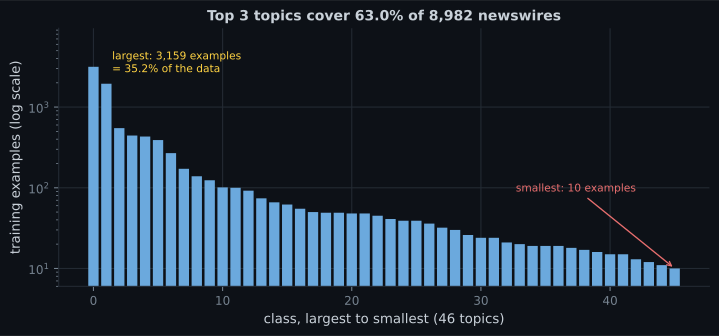
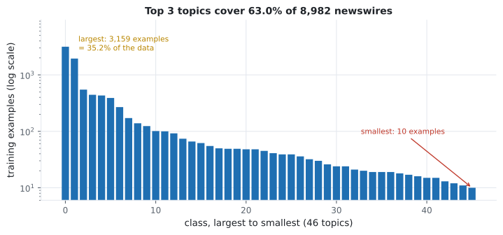
Going from 2 classes to 46 changes three lines of code — the output width, the activation, the loss — and it changes everything about how you should read the result. The IMDB dataset was exactly 50/50 balanced. Reuters has one topic holding 35% of the data and another holding 10 examples, and that single fact makes accuracy a misleading number.

What you’ll learn

• Softmax derived from scratch, verified against Keras to 3.27e−08, plus why the max is subtracted before exponentiating.
• The two baselines: majority class 0.3620, uniform guessing 0.0217.
• Sparse integer labels versus one-hot: identical loss, 23× less memory.
• What a 4-unit bottleneck costs, measured: 0.7703 → 0.6207 test accuracy.
• Why 0.7703 accuracy sits alongside a macro-average recall of 0.3279 — and that 13 of 46 classes were never predicted once.
• How to trade coverage for reliability: abstain below 0.90 confidence and accuracy rises to 0.9389 on the 55% of newswires you keep.

46 classes, wildly unequal

Loading the newswires

from tensorflow import keras
import numpy as np
 
(raw_train, y_train), (raw_test, y_test) = keras.datasets.reuters.load_data(
    num_words=10000)
 
print(len(raw_train), len(raw_test))     # 8982 2246
print(int(y_train.max()) + 1)            # 46
print(np.bincount(y_train).max())        # 3159

The label distribution is the defining feature of this dataset:

Rank	Class id	Training examples	Share
1	3	3,159	0.3517
2	4	1,949	0.2170
3	19	549	0.0611
4	16	444	0.0494
5	1	432	0.0481
…	…	…	…
46	35	10	0.0011

figure Every class in the training set, largest to smallest matplotlib

The vertical axis is logarithmic — on a linear axis the last thirty bars would be invisible. The largest topic has 3,159 examples and the smallest has 10, a ratio of 316x, and the top three topics together account for 63.0% of all 8,982 newswires.

Two baselines follow directly:

Baseline	Test accuracy
always predict class 3	0.3620
uniform random over 46 classes	0.0217

Any accuracy under 0.3620 is worse than a model that ignores the input entirely. That is the number to keep in mind for the rest of this page.

Softmax: turning scores into a distribution

The output layer produces 46 raw scores. Softmax converts them into probabilities that sum to 1:

$$\text{softmax}(\mathbf{z})_i = \frac{e^{z_i}}{\sum_{j=1}^{K} e^{z_j}}$$

Exponentiating makes everything positive; dividing by the sum makes it total 1. Because $e^x$ grows so fast, softmax exaggerates differences — a score gap of 1 becomes a probability ratio of $e \approx 2.72$.

Worked on three scores by hand:

$z$	$e^z$	probability
2.0	7.389056	0.659001
1.0	2.718282	0.242433
0.1	1.105171	0.098566

Sum of probabilities: 1.000000. tf.nn.softmax returns the same three values to a maximum difference of 3.27e−08 (float32 rounding, not disagreement).

Why the max gets subtracted

Softmax is unchanged if you shift every score by the same constant $c$:

$$\frac{e^{z_i - c}}{\sum_j e^{z_j - c}} = \frac{e^{-c} e^{z_i}}{e^{-c} \sum_j e^{z_j}} = \frac{e^{z_i}}{\sum_j e^{z_j}}$$

That invariance is what makes the standard implementation safe. Computed naïvely on $\mathbf{z} = [1000, 1001, 1002]$, $e^{1000}$ overflows float64 and every probability comes back nan. Subtracting the max first gives $[0.090031, 0.244728, 0.665241]$ — the mathematically identical answer, with the largest exponent now $e^0 = 1$.

sketch Drag the scores, watch the distribution p5.js Pause Restart

Three raw output scores and their softmax. Drag any bar to change its score. The button adds 5 to all three at once — the probabilities do not move, because softmax is shift-invariant.

Labels: integers or one-hot

Two encodings, two matching losses, identical results:

The same loss, twice

integers = np.array([1, 0])
one_hot = np.eye(3, dtype="float32")[integers]
predictions = np.array([[0.1, 0.7, 0.2], [0.6, 0.3, 0.1]], dtype="float32")
 
keras.losses.sparse_categorical_crossentropy(integers, predictions)  # 0.433750
keras.losses.categorical_crossentropy(one_hot, predictions)          # 0.433750

The difference is 5.96e−08 — float32 rounding. The real difference is memory: one-hot labels for 8,982 rows and 46 classes cost 1,652,688 bytes against 71,856 for int64 integers, a factor of 23. At 46 classes that is trivial; at 50,000 vocabulary classes in a language model it is not, which is why sparse_categorical_crossentropy is the default choice.

The model, and one deliberate mistake

64-64-46, softmax out

model = keras.Sequential([
    keras.layers.Input((10000,)),
    keras.layers.Dense(64, activation="relu"),
    keras.layers.Dense(64, activation="relu"),
    keras.layers.Dense(46, activation="softmax"),
])
model.compile("rmsprop", "sparse_categorical_crossentropy",
              metrics=["accuracy"])

Layer	Parameters
Dense(64) on 10,000 inputs	$10{,}000 \times 64 + 64 = 640{,}064$
Dense(64) on 64 inputs	$64 \times 64 + 64 = 4{,}160$
Dense(46) on 64 inputs	$64 \times 46 + 46 = 2{,}990$
total	647,214

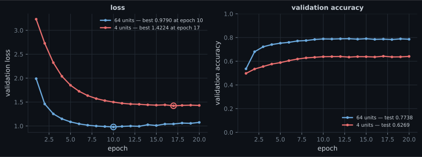
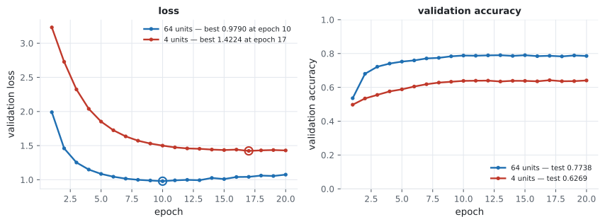
Now shrink the second hidden layer to 4 units and change nothing else:

figure Same input, same output, same everything but four numbers matplotlib

The 4-unit model reached 0.6269 test accuracy against the 64-unit model's 0.7738 — a loss of 0.1469 from one layer's width. It also took 17 epochs to reach its best validation loss instead of 10, and that best was 1.4224 against 0.9790.

Second hidden layer	Best val loss	At epoch	Val accuracy	Test accuracy
64 units	0.9790	10	0.7856	0.7738
4 units	1.4224	17	0.6408	0.6269

This is usually called an information bottleneck, and the phrase deserves care. Four real-valued numbers could in principle encode 46 labels — four float32s carry far more than the $\log_2 46 \approx 5.5$ bits required. The measured failure is not an information-theoretic impossibility; it is that gradient descent on a 4-dimensional ReLU representation does not find such a code. The layer’s output is non-negative and piecewise linear, the 46-way separation has to be linear in those four coordinates, and training lands in a much worse solution.

The lesson survives the correction: every layer’s width caps what the layers after it can distinguish, and no downstream capacity recovers what a narrow layer discarded. The practical rule is that intermediate layers should be comfortably wider than the number of output classes.

The accuracy number is hiding something

The 64-unit model reaches 0.7703 test accuracy (9 epochs, trained on 7,000 rows). Against the 0.3620 majority baseline that looks like a solid result. Then look per class:

Class id	Test examples	Recall
3	813	0.9668
4	474	0.8713
1	105	0.8000
19	133	0.7594
the 22 classes with ≤10 test examples (123 newswires)	123	0.1301

And the summary statistic that makes it unambiguous:

Metric	Value
accuracy (every newswire weighted equally)	0.7703
macro-average recall (every class weighted equally)	0.3279
classes never predicted even once	13 of 46

Accuracy 0.7703, macro recall 0.3279. Both are correct measurements of the same model. Accuracy is dominated by classes 3 and 4, which together are 57% of the test set and where the model scores 0.96 and 0.87. Averaged over classes instead of over rows, the model is barely better than a coin flip on the tail — and for 13 topics it has effectively learned that the safest move is to never guess them at all.

figure Where the errors actually go matplotlib

Row-normalised, so each row sums to 1 across all 46 predictions and the visible cells are the ten largest topics. Class 20 is the weakest of the ten at 0.44, and its errors are not random: 0.21 of them go to class 3 and 0.16 to class 19, the two largest topics available. When a model is unsure it drifts toward the classes it has seen most.

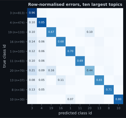
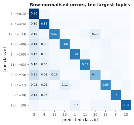
If your problem cares about the rare classes — fraud, rare diseases, uncommon faults — accuracy will tell you everything is fine while the model ignores exactly the cases you built it for. Report macro recall, per-class recall, or a confusion matrix alongside it.

Abstaining instead of guessing

Softmax gives a confidence with every prediction. Grouping the test set by that confidence:

Max softmax probability	Newswires	Accuracy in the band
[0.0, 0.4)	336	0.3661
[0.4, 0.7)	341	0.5718
[0.7, 0.9)	326	0.7515
[0.9, 1.0]	1,243	0.9389

Confidence is informative — it separates a 0.37 band from a 0.94 band — but it is not calibrated: mean confidence is 0.8567 when the model is right and still 0.5139 when it is wrong. Turn that into a policy by refusing to answer below a threshold:

Abstain below	Coverage	Newswires kept	Accuracy on kept
—	1.0000	2,246	0.7703
0.40	0.8504	1,910	0.8414
0.70	0.6986	1,569	0.8999
0.90	0.5534	1,243	0.9389
0.99	0.2235	502	0.9622

Answering only the 55% it is most sure about takes the model from 0.7703 to 0.9389 — without touching a single weight. In any workflow where a human can handle the rest, that trade is usually the whole product.

sketch Trade coverage for accuracy p5.js Pause Restart

Drag the threshold across the five measured cutoffs. Coverage is the share of the 2,246 test newswires the model still answers; accuracy is measured on that kept subset.

The whole pipeline

diagram Diagram mermaid

  flowchart TD
  A["8,982 newswires
integer sequences"] --> B["multi-hot
10,000 columns"]
  B --> C["Dense 64 relu"]
  C --> D["Dense 64 relu
never narrower than the class count"]
  D --> E["Dense 46 softmax
46 probabilities summing to 1"]
  E --> F["argmax -> predicted class"]
  E --> G["max -> confidence"]
  G --> H["below threshold?
abstain instead of guessing"]
  I["integer labels + sparse_categorical_crossentropy"] -.-> E

Pitfalls

• Reading accuracy alone on imbalanced data. 0.7703 accuracy and 0.3279 macro recall describe the same model. Only one of them notices that 13 classes are never predicted.
• Forgetting the majority-class baseline. Predicting class 3 every time scores 0.3620 here. Any result must be compared against that, not against 1/46.
• Making an intermediate layer narrower than the output. 4 units cost 0.1469 test accuracy against 64.
• Mismatching label encoding and loss. Integer labels with categorical_crossentropy (or one-hot with the sparse_ version) produces a shape error at best and a silently wrong loss at worst.
• Computing softmax without subtracting the max. $e^{1000}$ overflows to inf and every probability becomes nan.
• Treating softmax output as calibrated probability. Mean confidence was 0.5139 on the predictions that were wrong.
• Using softmax on the output layer and from_logits=True in the loss. The loss then exponentiates already-normalised probabilities. Pick one.

Recap

• Reuters has 46 topics, 8,982 training newswires, and a 316× ratio between the largest and smallest class.
• Softmax exponentiates and normalises; it is shift-invariant, which is exactly why implementations subtract the max before exponentiating.
• Sparse integer labels and one-hot labels give identical losses; integers cost 23× less memory here and far less on large label spaces.
• Narrowing the second hidden layer from 64 to 4 units cost 0.1469 test accuracy. Keep intermediate widths above the number of classes.
• Accuracy 0.7703 versus macro recall 0.3279 is the central lesson: on imbalanced data, always report a per-class view.
• Abstaining below 0.90 confidence raises accuracy to 0.9389 on the 55.3% of newswires the model still answers.

Next

The same three-step recipe once more, with a continuous target instead of a class — which changes the loss, the last layer, and how you have to validate when there are only 404 training rows: Predicting House Prices.

pch.quizTag pch.quizDefaultTitle

1. The model scores 0.7703 accuracy and 0.3279 macro-average recall. What is the difference between those two numbers measuring?

   A Macro recall is computed on the training set B Accuracy weights every newswire equally, so the two largest topics (57% of the test set) dominate it; macro recall weights every class equally, so the 44 small topics count as much as the big two C Macro recall is a stricter version of accuracy applied to the same rows D They differ only because of rounding
   pch.quizShowAnswer

   B — Accuracy weights every newswire equally, so the two largest topics (57% of the test set) dominate it; macro recall weights every class equally, so the 44 small topics count as much as the big two — The model gets 0.9668 recall on class 3 and 0.1301 on the 22 rarest classes. Row-weighted and class-weighted averages therefore tell opposite stories.

2. Why is 1/46 = 0.0217 the wrong baseline to compare a Reuters model against?

   A Because random guessing is never a valid baseline B Because the classes are heavily imbalanced: always predicting the largest class scores 0.3620, so that is the real bar to beat C Because 46 classes is too many for a baseline to be meaningful D Because accuracy is not defined for multiclass problems
   pch.quizShowAnswer

   B — Because the classes are heavily imbalanced: always predicting the largest class scores 0.3620, so that is the real bar to beat — Uniform guessing only makes sense as a baseline when the classes are uniform. Here the majority-class baseline is 17x higher.

3. Softmax implementations subtract the maximum score before exponentiating. What does that change?

   A It makes the largest probability bigger B Nothing mathematically — softmax is shift-invariant — but it prevents e^z from overflowing to infinity, which turns every probability into nan C It normalises the scores to have zero mean D It makes the gradient easier to compute
   pch.quizShowAnswer

   B — Nothing mathematically — softmax is shift-invariant — but it prevents e^z from overflowing to infinity, which turns every probability into nan — For z = [1000, 1001, 1002] the naive form returns nan; subtracting the max gives [0.090031, 0.244728, 0.665241].

4. Narrowing the second hidden layer from 64 to 4 units dropped test accuracy from 0.7738 to 0.6269. What is the precise reason?

   A Four float32 numbers cannot represent 46 distinct labels B Four numbers could encode 46 labels in principle, but gradient descent on a non-negative 4-dimensional ReLU representation does not find such a code, and no later layer can restore what that layer dropped C The 4-unit model has too few parameters to train at all D Softmax requires at least as many inputs as classes
   pch.quizShowAnswer

   B — Four numbers could encode 46 labels in principle, but gradient descent on a non-negative 4-dimensional ReLU representation does not find such a code, and no later layer can restore what that layer dropped — The failure is about what training finds, not about bits. The practical rule still holds: keep intermediate layers wider than the class count.

5. Refusing to predict when confidence is below 0.90 raised accuracy from 0.7703 to 0.9389. What was given up?

   A Nothing — this is free accuracy B Coverage: 44.7% of newswires now get no answer at all, so the gain is only useful if something else (a human, a fallback rule) handles them C The model had to be retrained on less data D The rare classes are no longer predicted
   pch.quizShowAnswer

   B — Coverage: 44.7% of newswires now get no answer at all, so the gain is only useful if something else (a human, a fallback rule) handles them — Selective prediction trades coverage for reliability. Always report both numbers — an accuracy figure without its coverage is meaningless.

🧪 Try It Yourself

pch.exerciseTag pch.exerciseTitle

pch.exerciseTag pch.exerciseTitle

pch.exerciseTag pch.exerciseTitle

pch.exerciseTag pch.exerciseTitle

pch.exerciseTag pch.exerciseTitle

pch.exerciseTag pch.exerciseTitle