Support Vector Machines (SVM)

What you’ll learn

why “the widest street” is a better objective than “any separating line”
the margin formula $2/\lVert\mathbf{w}\rVert$ , derived rather than quoted
a complete hard-margin SVM solved by hand on three points
hinge loss and the soft margin, and what CC actually buys
the kernel trick: non-linear boundaries without ever computing the new features
what gammagamma controls, and how RBF fails at both extremes

Intuition

Logistic regression finds a line that separates the classes. If the data is separable there are infinitely many such lines, and it has no principled reason to prefer one over another.

An SVM does. It looks for the line with the widest empty corridor around it — the one that stays as far as possible from the nearest point of either class. Intuitively, a boundary with room on both sides is more likely to survive contact with new data than one that skims past a training point.

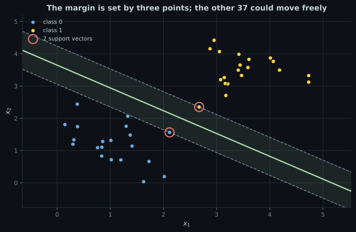
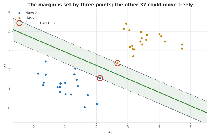
The remarkable consequence: only the points touching the corridor edge matter. Those are the support vectors, and every other point could be deleted without changing the model at all.

diagram Diagram mermaid

  flowchart LR
  D["Training data"] --> M["Find the widest corridor
separating the classes"]
  M --> SV["Points touching the edge
= support vectors"]
  M --> B["Boundary runs down the middle"]
  SV --> B
  X["Everything else"] -.->|"irrelevant"| B

The math

The margin

For a linear model $f(\mathbf{x}) = \mathbf{w}^\top\mathbf{x} + b$ , the distance from a point to the boundary $f(\mathbf{x}) = 0$ is

\text{distance} = \frac{\lvert \mathbf{w}^\top\mathbf{x} + b \rvert}{\lVert\mathbf{w}\rVert}

We are free to rescale $\mathbf{w}$ and $b$ together without moving the boundary, so fix the scale by requiring the closest points on each side to satisfy $\lvert f(\mathbf{x})\rvert = 1$ . Those points then sit at distance $1/\lVert\mathbf{w}\rVert$ , and the full corridor width is

\text{margin} = \frac{2}{\lVert\mathbf{w}\rVert}

Maximising the margin means minimising $\lVert\mathbf{w}\rVert$ , which gives the hard-margin problem:

\min_{\mathbf{w}, b} \frac{1}{2}\lVert\mathbf{w}\rVert^2 \quad\text{subject to}\quad y^{(i)}\left(\mathbf{w}^\top\mathbf{x}^{(i)} + b\right) \geq 1 \;\; \text{for all } i

with labels coded as $\pm 1$ . It is a convex quadratic program: one global optimum, no local minima.

Soft margin and hinge loss

Real data is not separable, and one mislabelled point would make the hard-margin problem infeasible. The soft margin introduces slack $\xi_i \geq 0$ and charges for it:

\min_{\mathbf{w}, b, \boldsymbol{\xi}} \; \frac{1}{2}\lVert\mathbf{w}\rVert^2 + C\sum_{i=1}^{m}\xi_i \quad\text{subject to}\quad y^{(i)}\left(\mathbf{w}^\top\mathbf{x}^{(i)} + b\right) \geq 1 - \xi_i,\;\; \xi_i \geq 0

Eliminating the slack variables turns this into an unconstrained problem with the hinge loss:

\min_{\mathbf{w}, b} \; \frac{1}{2}\lVert\mathbf{w}\rVert^2 + C\sum_{i=1}^{m}\max\!\left(0,\; 1 - y^{(i)}f(\mathbf{x}^{(i)})\right)

Read the hinge: a point that is correctly classified and outside the margin costs exactly zero. Only points inside or across the margin contribute anything, and those are the support vectors. That is the mechanism behind the sparsity.

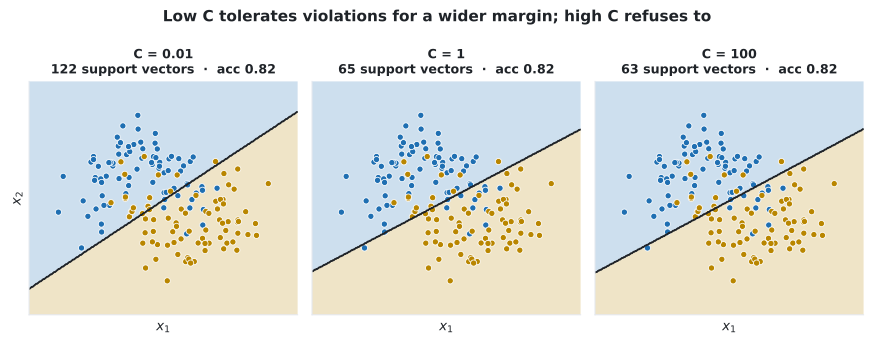
$C$ is the price of a violation. Large $C$ makes violations expensive, so the model narrows the margin to avoid them — low bias, high variance. Small $C$ tolerates violations for a wider corridor — high bias, low variance. Note that this is the same inverted convention as logistic regression: $C$ is the inverse of regularisation strength.

Worked example by hand

Three points, two classes, chosen so the whole problem is solvable on paper.

point	$x_1$	$x_2$	class $y$
A	1	1	−1
B	0	2	−1
C	3	3	+1

Step 1 — guess the direction from symmetry. A and B both lie on the line $x_1 + x_2 = 2$ , and C lies on $x_1 + x_2 = 6$ . The separating boundary must run parallel to both, so $\mathbf{w} \propto (1, 1)$ . Write $\mathbf{w} = (a, a)$ .

Step 2 — impose the margin conditions. The support vectors must satisfy $f = \pm 1$ :

f(C) = 3a + 3a + b = +1 \qquad f(A) = a + a + b = -1

Step 3 — solve. Subtracting gives $4a = 2$ , so $a = 0.5$ , and then $b = -1 - 2(0.5) = -2$ .

\mathbf{w} = (0.5,\ 0.5), \qquad b = -2

Step 4 — check B. $f(B) = 0.5(0) + 0.5(2) - 2 = -1$ . Exactly on the margin, so B is a support vector too — all three points are.

Step 5 — the margin width.

\lVert\mathbf{w}\rVert = \sqrt{0.5^2 + 0.5^2} = \frac{1}{\sqrt{2}} \approx 0.7071, \qquad \text{margin} = \frac{2}{0.7071} \approx 2.828

Step 6 — the boundary as a line. $0.5x_1 + 0.5x_2 - 2 = 0$ , that is $x_1 + x_2 = 4$ — precisely the perpendicular bisector between the two class lines, as symmetry demanded.

SVC(kernel="linear", C=1000)SVC(kernel="linear", C=1000) on these three points returns $\mathbf{w} = (0.5002, 0.4995)$ and $b = -1.9993$ , converging to the hand solution to three decimals.

See it move

The hand solution came from symmetry. The sketch solves the same problem by search: for every candidate direction it projects all points onto that direction, finds the widest empty corridor between the classes, and keeps the direction where that corridor is widest. In two dimensions that is the hard-margin SVM, exactly — no optimiser required.

Drag any point. The reported $\mathbf{w}$ , $b$ and margin update live, and the points that touch the corridor edge are circled: those are the support vectors.

sketch Drag a point, watch the margin re-solve p5.js

Three points from the worked example, draggable. For each of 360 candidate directions the sketch measures the gap between the classes and keeps the widest, then reports w, b and the margin width. Points touching the corridor edge are circled as support vectors; dragging a non-support point changes nothing until it enters the corridor.

Two behaviours worth provoking deliberately. Drag the fourth point around outside the corridor and every number on the panel stays frozen — that is the sparsity property, stated as a fact you can feel rather than a theorem. Drag it into the corridor and the whole solution snaps to a new direction, because a single point can now be the binding constraint. That sensitivity is why hard margins are rarely used on real data, and it is what $C$ softens.

Scatter of two classes with a solid decision boundary, two dashed margin lines forming a shaded corridor, and three circled points sitting exactly on the margin edges. — Circled points are the support vectors. Every other point sits outside the corridor, contributes zero hinge loss, and could be deleted without changing the model.

Soft margin in practice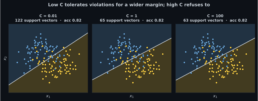

Three panels of the same overlapping dataset with linear SVM boundaries at C equal to 0.01, 1 and 100, with the number of support vectors falling as C rises. — At C = 0.01 almost every point is a support vector and the margin is enormous. At C = 100 the model keeps only a handful and squeezes the corridor to avoid violations.

Reading the plot

Support vector count is a regularisation diagnostic. On the iris virginica problem, C=0.01C=0.01 keeps all 100 points as support vectors; C=1C=1 keeps 26; C=100C=100 keeps 12. A model whose support vectors are most of the training set is heavily regularised.
Accuracy barely moves across two orders of magnitude of $C$ here (0.96, 0.95, 0.96). $C$ matters most when the classes genuinely overlap.
Fewer support vectors also means faster prediction, since prediction cost scales with their number.

The kernel trick

Suppose the data is not linearly separable in its original space. Map it into a higher-dimensional space where it is:

\mathbf{x} \mapsto \phi(\mathbf{x})

The catch is that a useful $\phi$ can be enormous, sometimes infinite-dimensional. The kernel trick avoids ever building it. The SVM’s dual formulation touches the data only through inner products $\phi(\mathbf{a})^\top\phi(\mathbf{b})$ , and for many useful maps that inner product has a closed form computable in the original space:

K(\mathbf{a}, \mathbf{b}) = \phi(\mathbf{a})^\top\phi(\mathbf{b})

Kernel	$K(\mathbf{a}, \mathbf{b})$	Effective feature space
Linear	$\mathbf{a}^\top\mathbf{b}$	The original features
Polynomial	$(\gamma\,\mathbf{a}^\top\mathbf{b} + r)^{d}$	All monomials up to degree $d$
RBF (Gaussian)	$\exp\!\left(-\gamma\lVert\mathbf{a} - \mathbf{b}\rVert^2\right)$	Infinite-dimensional
Sigmoid	$\tanh(\gamma\,\mathbf{a}^\top\mathbf{b} + r)$	Neural-network-like

The RBF kernel corresponds to an infinite-dimensional feature map, yet costs one exponential per pair. That is the trick: the space is never constructed, only its geometry is used.

What gamma does

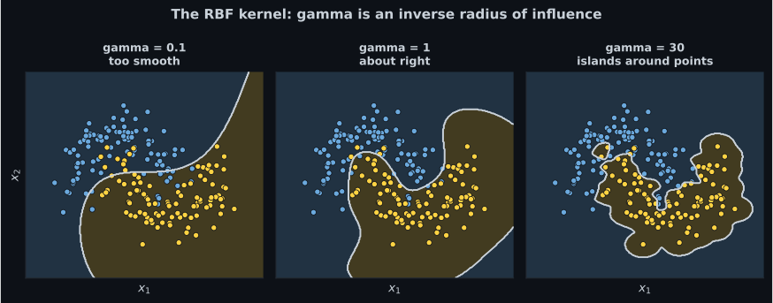
K(\mathbf{a}, \mathbf{b}) = \exp\!\left(-\gamma\lVert\mathbf{a} - \mathbf{b}\rVert^2\right)

$\gamma$ is an inverse radius of influence. Small $\gamma$ means a single training point affects predictions far away, giving smooth boundaries. Large $\gamma$ means influence dies off almost immediately, and the model builds a tight bubble around each training point.

Three panels of the same crescent-shaped dataset with RBF SVM boundaries at gamma equal to 0.1, 1 and 30. The first is nearly linear, the second follows the crescents, and the third forms isolated islands around individual points. — At gamma = 30 the model reaches 0.99 training accuracy by drawing a bubble around each point — the classic signature of overfitting with an RBF kernel.

CC and gammagamma interact, so tune them together on a log grid rather than one at a time:

svm_grid.py

import numpy as np
from sklearn.datasets import load_breast_cancer
from sklearn.model_selection import GridSearchCV, train_test_split
from sklearn.pipeline import make_pipeline
from sklearn.preprocessing import StandardScaler
from sklearn.svm import SVC
 
X, y = load_breast_cancer(return_X_y=True)
y = 1 - y
X_tr, X_te, y_tr, y_te = train_test_split(
    X, y, test_size=0.3, random_state=0, stratify=y
)
 
pipe = make_pipeline(StandardScaler(), SVC(kernel="rbf"))
grid = GridSearchCV(
    pipe,
    {"svc__C": np.logspace(-2, 3, 6), "svc__gamma": np.logspace(-4, 1, 6)},
    cv=5,
    n_jobs=-1,
)
grid.fit(X_tr, y_tr)
 
print("best params:", grid.best_params_)
print(f"CV accuracy   {grid.best_score_:.4f}")
print(f"test accuracy {grid.score(X_te, y_te):.4f}")

svm_grid.py

import numpy as np
from sklearn.datasets import load_breast_cancer
from sklearn.model_selection import GridSearchCV, train_test_split
from sklearn.pipeline import make_pipeline
from sklearn.preprocessing import StandardScaler
from sklearn.svm import SVC
 
X, y = load_breast_cancer(return_X_y=True)
y = 1 - y
X_tr, X_te, y_tr, y_te = train_test_split(
    X, y, test_size=0.3, random_state=0, stratify=y
)
 
pipe = make_pipeline(StandardScaler(), SVC(kernel="rbf"))
grid = GridSearchCV(
    pipe,
    {"svc__C": np.logspace(-2, 3, 6), "svc__gamma": np.logspace(-4, 1, 6)},
    cv=5,
    n_jobs=-1,
)
grid.fit(X_tr, y_tr)
 
print("best params:", grid.best_params_)
print(f"CV accuracy   {grid.best_score_:.4f}")
print(f"test accuracy {grid.score(X_te, y_te):.4f}")

Scaling is mandatory

The RBF kernel is a function of $\lVert\mathbf{a}-\mathbf{b}\rVert^2$ , so — exactly as with KNN — a feature with a large numeric range dominates the distance and the others stop mattering. The linear kernel is affected too, because the $\lVert\mathbf{w}\rVert^2$ penalty charges by coefficient size, and coefficient size depends on feature units.

Always make_pipeline(StandardScaler(), SVC(...))make_pipeline(StandardScaler(), SVC(...)).

SVM for regression

The same machinery, inverted. Instead of keeping points outside a margin, SVR asks for them to be inside an $\epsilon$ -wide tube, and only points outside the tube incur a cost:

\text{loss} = \max\!\left(0,\; \lvert y - f(\mathbf{x})\rvert - \epsilon\right)

Widening $\epsilon$ makes the tube more forgiving and produces fewer support vectors. SVRSVR and LinearSVRLinearSVR implement it, and everything about scaling and kernels carries over unchanged.

algorithmSupport Vector MachineSupervised · Classification and Regression · Max-margin

APIsklearn.svm.SVC / LinearSVC / SVR

Assumes

A margin exists in the original space, or in some kernel-induced space
Features are on comparable scales
The dataset is small enough for a quadratic-program solver
You do not need calibrated probabilities directly from the model

Cost

train: O(m² · n) to O(m³ · n)
predict: O(n · number of support vectors)
memory: O(support vectors × n)

m = samples, n = features; the quadratic-to-cubic training cost is why SVC struggles past roughly 50,000 rows

Hyperparameters that matter

Cdefault 1.0Price of a margin violation. Large C narrows the margin and overfits; small C widens it and underfits. Inverse of regularisation strength.
kerneldefault rbf'linear' for wide, sparse data such as text; 'rbf' as the general-purpose default; 'poly' when interactions of a known degree matter.
gammadefault scaleRBF radius of influence, inverted. Large gamma builds islands around individual points.
class_weightdefault None'balanced' reweights the hinge loss by inverse class frequency — the first move on imbalanced data.
probabilitydefault FalseEnables predict_proba via Platt scaling, at the cost of an internal 5-fold cross-validation. Slow, and the probabilities are only approximately calibrated.

Reach for it when

The dataset is small to medium with many features — text classification is the classic case
The boundary is non-linear but smooth
You want a margin-based model that is robust to points far from the boundary
Feature count exceeds sample count, where SVMs remain well behaved

Look elsewhere when

There are hundreds of thousands of rows — training is quadratic to cubic
You need calibrated probabilities without extra work
You need to explain the model to a non-technical audience
Features cannot be scaled

Pitfalls

Compare

Model	Boundary	Scales to big data	Probabilities	Sensitive to outliers
SVM (RBF)	Smooth, non-linear	Poorly	Only via Platt scaling	Low — far points cost zero
SVM (linear)	Linear, max-margin	Moderately, via `LinearSVCLinearSVC`	Only via Platt scaling	Low
Logistic Regression	Linear	Well	Yes, calibrated	Moderate
KNN	Arbitrarily local	Poorly at predict time	Coarse	Moderate
Random Forest	Axis-aligned, complex	Well	Reasonable	Low

The hinge loss is what makes SVMs robust: a point far on the correct side contributes exactly zero, whereas log loss keeps rewarding extra confidence forever.

quizCheck yourself

Why maximise the margin instead of accepting any separating line?
Show answer
B — A boundary with clearance on both sides is more likely to generalise than one that skims a training point — Among infinitely many separating lines, the widest-corridor one has the most room for new points to fall in without crossing. That is the geometric expression of a low-variance choice.
What does it mean that only support vectors matter?
Show answer
B — Points outside the margin contribute zero hinge loss, so deleting them leaves the fitted boundary unchanged — The hinge loss max(0, 1 - y·f(x)) is exactly zero for any correctly classified point outside the margin. Those points exert no force on the optimisation.
What is the kernel trick actually avoiding?
Show answer
B — Explicitly constructing the high-dimensional feature map — the optimisation only ever needs inner products, which the kernel computes directly — The dual problem touches the data only through inner products of mapped vectors. A kernel returns that inner product in the original space, so an infinite-dimensional map costs one exponential.
Your RBF SVM has training accuracy 0.99 and test accuracy 0.72. Which knob do you turn first?
Show answer
B — Decrease gamma and decrease C — both are currently letting the model build bubbles around individual points — That gap is textbook RBF overfitting. Large gamma shrinks each point's influence to a bubble, and large C refuses any margin violation. Reduce both, and grid-search the pair together.

🧪 Try It Yourself

Exercise 1 – Recover the hand-solved SVM

Exercise 2 – Compute the margin width

Exercise 3 – Count support vectors as C changes

Exercise 4 – Watch gamma overfit

Exercise 5 – Widen the epsilon tube in SVR

Recap

The margin is $2/\lVert\mathbf{w}\rVert$ , so maximising it means minimising $\lVert\mathbf{w}\rVert$ subject to every point being correctly classified by at least 1.
Hand-solved on three points: $\mathbf{w} = (0.5, 0.5)$ , $b = -2$ , margin 2.828, boundary $x_1 + x_2 = 4$ — and SVCSVC reproduces it to three decimals.
The hinge loss is exactly zero outside the margin, which is why only support vectors matter.
$C$ is the price of a violation: large $C$ narrows the margin, small $C$ widens it. On iris, $C$ from 0.01 to 100 takes the support vector count from 100 to 12.
The kernel trick replaces an explicit high-dimensional map with an inner product computed in the original space; RBF corresponds to an infinite-dimensional space.
$\gamma$ is an inverse radius of influence — large values build a bubble around each point and overfit.
Always scale, and always tune $C$ and $\gamma$ together.

Exercise 6 – Solve the hard margin by brute force

Continue to Decision Trees - Entropy and Gini Impurity — a model that needs no scaling, no distance metric and no kernel, and that you can read out loud as a list of rules.

If this helped you, consider buying me a coffee ☕

Buy me a coffee