Higher-Order Derivatives

§5.7 is two pages long, and it opens with a reason rather than a definition:

Sometimes, we are interested in derivatives of higher order, e.g., when we want to use Newton’s Method for optimization, which requires second-order derivatives.

That is the whole motivation, and it is worth taking seriously before the notation arrives. Every method in §5.6 computes a gradient. A gradient tells you which way is downhill and how steeply. It does not tell you how far to go, and it does not tell you whether the flat spot you have arrived at is the bottom of a valley, the top of a hill, or a mountain pass. Those are second-order questions, and second derivatives are the answer to all three.

What you’ll learn

• The book’s notation for higher-order partials, and why the order of the subscripts is a real distinction and not decoration.
• Equation 5.146, Schwarz’s theorem — and the hypothesis in it that everyone drops, with the function that punishes you for dropping it.
• Equation 5.147, the Hessian, and why symmetry is the property that lets §4.2’s spectral theorem do the classifying.
• What “the Hessian measures the curvature of the function locally” means as an equation: the second derivative along a unit direction $\mathbf{d}$ is exactly $\mathbf{d}^\top H \mathbf{d}$, and its extremes over all $\mathbf{d}$ are the eigenvalues.
• The second-order test, its three verdicts, and the fourth outcome — silence — which is where three different functions with one shared Hessian part company.
• Newton’s method, measured: quadratic convergence, 8 steps against 426, no learning rate — and the two ways it fails that gradient descent does not.
• The book’s Remark: for a vector field the Hessian is an $(m \times n \times n)$ tensor, which is why a loss is always a scalar.

Intuition: slope says where, curvature says what

Stand on a hillside in fog with a spirit level. The level tells you the slope under your feet — that is the gradient, and it is enough to walk downhill. Walk until the bubble centres, and now the level is useless: it reads flat at the bottom of a valley, flat at the summit, and flat in the middle of a pass.

To tell those apart you need a second instrument, one that measures how the slope changes as you step. Take one step north and re-read the level: if the slope tilts back toward you, the ground curves upward in that direction. Do it east as well. Do it along every compass bearing, and you have the whole local shape.

The Hessian is that instrument, and it fits in four numbers because curvature in every direction is determined by curvature along two — a fact that is not obvious and is exactly what the eigendecomposition is for.

diagram Diagram mermaid

  flowchart TD
  F["f : R^n -> R"] --> G["grad f (Eq 5.40)
1 x n, the slope"]
  F --> H["H (Eq 5.147)
n x n, the curvature"]
  G --> C{"grad f = 0 ?"}
  C -->|"no"| W["keep walking downhill"]
  C -->|"yes"| Q["a critical point:
the gradient is finished talking"]
  H --> S["symmetric, by Eq 5.146"]
  S --> E["real eigenvalues,
orthonormal eigenvectors (§4.2)"]
  Q --> E
  E -->|"all lambda > 0"| MIN["minimum"]
  E -->|"all lambda < 0"| MAX["maximum"]
  E -->|"mixed signs"| SAD["saddle point"]
  E -->|"some lambda = 0"| SIL["SILENT: ask a higher derivative"]
  H --> N["Newton: x - H^-1 grad f"]
  E --> K["kappa = lambda_max / lambda_min
the rate gradient descent pays"]

The math

Notation, and why the order matters

For $f : \mathbb{R}^2 \to \mathbb{R}$ of two variables $x, y$, the book fixes four pieces of notation:

Notation	Meaning
$\dfrac{\partial^2 f}{\partial x^2}$	differentiate twice with respect to $x$
$\dfrac{\partial^n f}{\partial x^n}$	the $n$th partial derivative with respect to $x$
$\dfrac{\partial^2 f}{\partial y\,\partial x} = \dfrac{\partial}{\partial y}\!\left(\dfrac{\partial f}{\partial x}\right)$	$x$ first, then $y$
$\dfrac{\partial^2 f}{\partial x\,\partial y}$	$y$ first, then $x$

Read the last two carefully: the operator closest to $f$ acts first, so the subscripts are read right to left. It is a genuinely confusing convention, and the only mercy is that Equation 5.146 makes the distinction moot for the functions you will actually meet — which is precisely why so many people never notice that they had it backwards.

Equation 5.146, and the hypothesis in it

If $f(x, y)$ is a twice (continuously) differentiable function, then

$$\frac{\partial^2 f}{\partial x\,\partial y} = \frac{\partial^2 f}{\partial y\,\partial x} \tag{5.146}$$

The order of differentiation does not matter. Almost every statement of this result you will see in an ML context drops the hypothesis and says “mixed partials commute”, full stop. They do not, in general. The counterexample is standard and short:

$$g(x, y) = \begin{cases} \dfrac{xy\left(x^2 - y^2\right)}{x^2 + y^2} & (x, y) \neq (0, 0) \\[6pt] 0 & (x, y) = (0, 0) \end{cases}$$

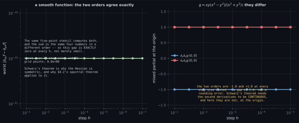
Both mixed partials exist at the origin. They are $-1$ and $+1$. The from scratch section measures them, and the gap is exactly $2$ at every step size — not a small numerical discrepancy, a whole integer. What fails is not differentiability, it is continuity of the second derivatives at the origin, which is the clause the short version of the theorem throws away.

Equation 5.147, the Hessian

Collect all four second partials:

$$H = \begin{bmatrix} \dfrac{\partial^2 f}{\partial x^2} & \dfrac{\partial^2 f}{\partial x\,\partial y} \\[10pt] \dfrac{\partial^2 f}{\partial x\,\partial y} & \dfrac{\partial^2 f}{\partial y^2} \end{bmatrix} \tag{5.147}$$

The book writes it with the same entry in both off-diagonal slots, which is Equation 5.146 already applied. The Hessian is denoted $\nabla^2_{x,y} f(x, y)$. Generally, for $\mathbf{x} \in \mathbb{R}^n$ and $f : \mathbb{R}^n \to \mathbb{R}$, $H$ is an $n \times n$ matrix, and

The Hessian measures the curvature of the function locally around $(x, y)$.

That sentence is the payload of the section, and the next subsection turns it into something you can check.

What “measures the curvature” actually says

Take a unit direction $\mathbf{d}$ and walk along it: define $\varphi(t) = f(\mathbf{x} + t\mathbf{d})$. Differentiate twice by the chain rule of §5.2:

$$\varphi'(t) = \nabla f(\mathbf{x} + t\mathbf{d})\,\mathbf{d}, \qquad \varphi''(t) = \mathbf{d}^\top H(\mathbf{x} + t\mathbf{d})\,\mathbf{d}$$

so at $t = 0$:

$$\left.\frac{\mathrm{d}^2}{\mathrm{d}t^2} f(\mathbf{x} + t\mathbf{d})\right|_{t=0} = \mathbf{d}^\top H \mathbf{d}$$

That is the precise version of the sentence. The curvature along $\mathbf{d}$ is a quadratic form in $\mathbf{d}$, and because $H$ is symmetric, §4.2 tells you everything about that form at once: it has an orthonormal eigenbasis, and over all unit $\mathbf{d}$,

$$\lambda_{\min} \;\le\; \mathbf{d}^\top H \mathbf{d} \;\le\; \lambda_{\max}$$

with both bounds attained, along the corresponding eigenvectors. Two numbers pin down the curvature in every one of infinitely many directions. That is the content of “the Hessian measures curvature”, and the curvature sweep below draws it as a rosette and checks it against a measured second difference in all 360 directions.

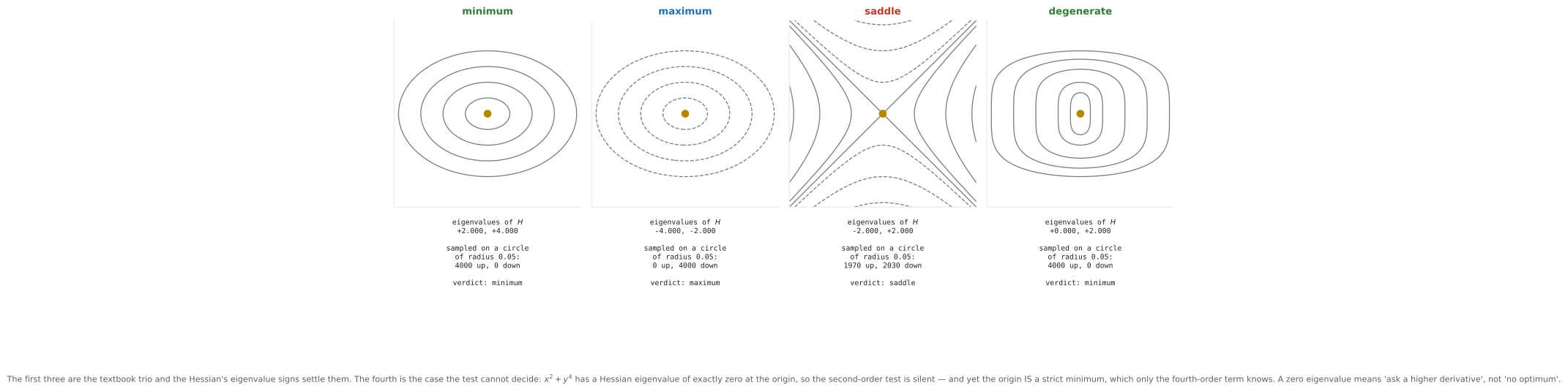
The second-order test, and its fourth outcome

At a critical point ($\nabla f = \mathbf{0}$) the signs of the eigenvalues classify it:

Eigenvalues of $H$	Quadratic form	Critical point	Shape
all $> 0$	positive definite	strict minimum	bowl
all $< 0$	negative definite	strict maximum	dome
mixed signs	indefinite	saddle point	pass
some $= 0$	semidefinite	the test says nothing	—

The fourth row is not an edge case to be waved past. Here are three functions:

$$x_1^2 + x_2^4, \qquad x_1^2 + x_2^3, \qquad x_1^2 - x_2^4$$

All three have gradient $\mathbf{0}$ at the origin. All three have the same Hessian there,

$$H = \begin{bmatrix} 2 & 0 \\ 0 & 0 \end{bmatrix}$$

and the origin is a strict minimum for the first and not an optimum at all for the other two. No second-order information can separate them, because they do not differ at second order. A zero eigenvalue means ask a higher derivative, not no optimum.

Newton’s method

The reason the book raises second derivatives at all. Model $f$ near $\mathbf{x}$ by its second-order Taylor polynomial — the subject of the next page — and jump to the minimum of the model rather than taking a small step downhill:

$$\mathbf{x}_{\text{new}} = \mathbf{x} - H^{-1} \nabla f(\mathbf{x})^\top$$

Three consequences, all measured below:

1. On a quadratic it is exact in one step, whatever the conditioning, because there the model is $f$.
2. Near a minimum it converges quadratically — the error roughly squares each step. Measured: $1.08\text{e-}01 \to 9.8\text{e-}03 \to 8.1\text{e-}05 \to 5.5\text{e-}09$.
3. It has no learning rate. The Hessian supplies the scale. Measured on the same problem: 8 Newton steps against 426 gradient-descent steps, and three of the four step sizes tried diverged outright.

The price is an $n \times n$ linear solve every step, which is why large models use first-order methods with cheap curvature proxies (L-BFGS’s low-rank approximation, Adam’s diagonal one) instead.

Newton’s method solves the wrong problem, correctly

$\mathbf{x} - H^{-1}\nabla f$ is derived from $\nabla f = \mathbf{0}$. It finds critical points, with no preference among them. On $f = x_1^2 - x_2^2$ one Newton step from anywhere lands exactly on the saddle — measured below as 0.0e+0. Gradient descent, which only ever goes downhill, walks away from the same point. Second-order information is strictly more information, and it is not automatically better behaved.

Vector-valued functions

The book closes §5.7 with a Remark: if $f : \mathbb{R}^n \to \mathbb{R}^m$ is a vector field, the Hessian is an $(m \times n \times n)$ tensor — one $n \times n$ Hessian per output component, stacked. Measured for $f : \mathbb{R}^2 \to \mathbb{R}^3$ below: shape $(3, 2, 2)$, each slice symmetric, matching the analytic tensor to $1.2\text{e-}08$.

There is no “eigenvalue of a tensor” to read a verdict from. Classification is a scalar-output idea — which is one concrete reason a training objective is always collapsed to a single number before anyone differentiates it twice.

From the book

Mathematics for Machine Learning, §5.7. The motivation for higher-order derivatives is Newton’s method (citing Nocedal and Wright, 2006). The four notational conventions for $\partial^2 f / \partial x^2$, $\partial^n f / \partial x^n$, $\partial^2 f / \partial y \partial x$ and $\partial^2 f / \partial x \partial y$ are stated with the “closest to $f$ acts first” reading. Equation 5.146 gives the commutation of mixed partials for a twice continuously differentiable $f$; Equation 5.147 defines the Hessian matrix, notes it is symmetric, that it is denoted $\nabla^2_{x,y} f(x,y)$, that it is $n \times n$ in general, and that it “measures the curvature of the function locally”. The closing Remark gives the $(m \times n \times n)$ tensor for a vector field. The book defers the classification test and Newton’s method themselves to Chapter 7.

Worked example by hand

Continue the book’s Example 5.7 from §5.2:

$$f(x_1, x_2) = x_1^2 x_2 + x_1 x_2^3$$

§5.2 found the gradient. Differentiate each component again. Start from

$$\frac{\partial f}{\partial x_1} = 2x_1x_2 + x_2^3, \qquad \frac{\partial f}{\partial x_2} = x_1^2 + 3x_1x_2^2$$

Step 1 — differentiate the first partial with respect to $x_1$. Treat $x_2$ as a constant. $2x_1x_2$ differentiates to $2x_2$; $x_2^3$ has no $x_1$ in it, so it goes to zero:

$$\frac{\partial^2 f}{\partial x_1^2} = 2x_2$$

Step 2 — differentiate the first partial with respect to $x_2$. Now $x_1$ is the constant. $2x_1x_2 \to 2x_1$, and $x_2^3 \to 3x_2^2$:

$$\frac{\partial^2 f}{\partial x_2\,\partial x_1} = 2x_1 + 3x_2^2$$

Step 3 — the other order, as a check. Differentiate $\partial f/\partial x_2 = x_1^2 + 3x_1x_2^2$ with respect to $x_1$: $x_1^2 \to 2x_1$ and $3x_1x_2^2 \to 3x_2^2$, so

$$\frac{\partial^2 f}{\partial x_1\,\partial x_2} = 2x_1 + 3x_2^2$$

Same expression. That is Equation 5.146 for this function, verified rather than assumed — and here the verification costs one line, which is the usual situation.

Step 4 — the last entry. $\partial f/\partial x_2 = x_1^2 + 3x_1x_2^2$ differentiated with respect to $x_2$: the first term dies and the second gives

$$\frac{\partial^2 f}{\partial x_2^2} = 6x_1x_2$$

Step 5 — assemble Equation 5.147.

$$H(x_1, x_2) = \begin{bmatrix} 2x_2 & 2x_1 + 3x_2^2 \\ 2x_1 + 3x_2^2 & 6x_1x_2 \end{bmatrix}$$

Unlike a quadratic’s, this Hessian is not constant — the curvature genuinely changes from point to point — and it is not diagonal, so the two variables are coupled.

Step 6 — evaluate at $(1, 1)$.

$$H(1, 1) = \begin{bmatrix} 2 & 5 \\ 5 & 6 \end{bmatrix}, \qquad \operatorname{tr} H = 8, \qquad \det H = 12 - 25 = -13$$

The determinant is the product of the eigenvalues and it is negative, so the eigenvalues have opposite signs — you can read “indefinite” off the determinant without computing either eigenvalue. For the record they are

$$\lambda = \frac{8 \pm \sqrt{16 + 100}}{2} = 4 \pm \sqrt{29} \approx -1.385165,\; 9.385165$$

Quantity	By hand	Differenced, $h = 10^{-4}$
$\partial^2 f/\partial x_1^2$	$2$	$2.00000003$
$\partial^2 f/\partial x_1 \partial x_2$	$5$	$5.00000001$
$\partial^2 f/\partial x_2 \partial x_1$	$5$	$5.00000001$
$\partial^2 f/\partial x_2^2$	$6$	$6.00000001$
worst gap	—	$3.2 \times 10^{-8}$

One thing this example is not

$\nabla f(1,1) = \begin{bmatrix} 3 & 4 \end{bmatrix} \neq \mathbf{0}$, so $(1,1)$ is not a critical point. The eigenvalues above describe the curvature there; they are not a verdict about an optimum, because there is no optimum at $(1,1)$ to have a verdict about. Reading “saddle” off an indefinite Hessian at a non-critical point is a common and meaningless move.

See it move

fieldA saddle, built from four difference stencilsthe Hessian, §5.7

H at (0, 0) — analytic, then by second differences at h = 1e-4

200-2

2.0000000.0000000.000000-2.000000

f(x) 0|grad f| 0.0e+0lambda_min -2lambda_max 2trace 0det -4condition number singular

grad f at this point [0.000, 0.000], norm 0.0e+0

1d2f/dx1^2  = [ f(x1+h, x2) - 2 f(x) + f(x1-h, x2) ] / h^22d2f/dx1dx2 = [ f(++) - f(+-) - f(-+) + f(--) ] / (4 h^2)3 4H = [ d2f/dx1^2    d2f/dx1dx2 ]                              # Eq 5.1475    [ d2f/dx2dx1   d2f/dx2^2  ]      symmetric by Eq 5.1466 7eigvalsh(H) -> curvature along the principal axes    # spectral thm, §4.28d^T H d     -> curvature along any unit d9 10x <- x - H^-1 grad f          # Newton, the reason §5.7 exists

The function is a mountain pass. Uphill along x1, downhill along x2, and flat along the two diagonals where the curvature cancels exactly. The gradient at (0, 0) is exactly zero — and that is all a first-order condition can tell you. It is the same zero at a minimum, a maximum and a saddle.

Play‹›1/7⟲

Seven frames: the point, the four entries, what the symmetry check can and cannot prove, the eigendecomposition, the curvature rosette, the verdict against a sampled ground truth, and one Newton step. Stop on the rosette — the dashed curve is a measured second difference lying on top of the analytic d-transpose-H-d.

fieldThe case the test cannot decidethe Hessian, §5.7

H at (0, 0) — analytic, then by second differences at h = 1e-4

2000

2.0000000.0000000.0000002.000000e-8

f(x) 0|grad f| 0.0e+0lambda_min 0lambda_max 2trace 2det 0condition number singular

grad f at this point [0.000, 0.000], norm 0.0e+0

1d2f/dx1^2  = [ f(x1+h, x2) - 2 f(x) + f(x1-h, x2) ] / h^22d2f/dx1dx2 = [ f(++) - f(+-) - f(-+) + f(--) ] / (4 h^2)3 4H = [ d2f/dx1^2    d2f/dx1dx2 ]                              # Eq 5.1475    [ d2f/dx2dx1   d2f/dx2^2  ]      symmetric by Eq 5.1466 7eigvalsh(H) -> curvature along the principal axes    # spectral thm, §4.28d^T H d     -> curvature along any unit d9 10x <- x - H^-1 grad f          # Newton, the reason §5.7 exists

The function is the case the second-order test cannot decide. One eigenvalue is exactly zero, so the Hessian is singular and says nothing about the x2 direction — and yet the origin IS a strict minimum, which only the fourth-order term knows. The gradient at (0, 0) is exactly zero — and that is all a first-order condition can tell you. It is the same zero at a minimum, a maximum and a saddle.

Play‹›1/7⟲

x1 squared plus x2 to the fourth. One eigenvalue is exactly zero, so the second-order test is silent — and the origin is a strict minimum anyway. Watch the stencil ladder: the exact zero measures as 2 h-squared, which is POSITIVE, so a naive positive-definiteness test gets the right answer here for entirely the wrong reason.

fieldExample 5.7's Hessian, which is neither constant nor diagonalthe Hessian, §5.7

H at (1, 1) — analytic, then by second differences at h = 1e-4

2556

2.0000005.0000005.0000006.000000

f(x) 2|grad f| 5.0e+0lambda_min -1.385165lambda_max 9.385165trace 8det -13condition number singular

grad f at this point (not critical) [3.000, 4.000], norm 5.0e+0

1d2f/dx1^2  = [ f(x1+h, x2) - 2 f(x) + f(x1-h, x2) ] / h^22d2f/dx1dx2 = [ f(++) - f(+-) - f(-+) + f(--) ] / (4 h^2)3 4H = [ d2f/dx1^2    d2f/dx1dx2 ]                              # Eq 5.1475    [ d2f/dx2dx1   d2f/dx2^2  ]      symmetric by Eq 5.1466 7eigvalsh(H) -> curvature along the principal axes    # spectral thm, §4.28d^T H d     -> curvature along any unit d9 10x <- x - H^-1 grad f          # Newton, the reason §5.7 exists

The function is the surface §5.2 built its gradient on, now differentiated twice. Here the Hessian is not constant and not diagonal, so the curvature genuinely depends on direction and the off-diagonal entry is what couples the two variables. At (1, 1) the gradient is [3.000, 4.000], so this is not a critical point — the Hessian here is still the local curvature, it just is not classifying an optimum.

Play‹›1/7⟲

The same surface §5.2 built its gradient on. The off-diagonal entry is 5, and it is what tips the curvature range out to minus 1.39 and plus 9.39. The last frame is the warning: at an indefinite point the Newton step is not a descent step, and here it lands FARTHER from the reference point than the gradient step does.

sketch Curvature in every direction p5.js Pause Restart

Drag the three entries of a symmetric H. The rosette is the curvature d-transpose-H-d as the direction d sweeps the circle: green where the surface bends up along that direction, red where it bends down. The rosette's widest and narrowest reaches are the eigenvalues, and the verdict follows from their signs alone.

sketch Why the test goes silent p5.js Pause Restart

f = x1 squared plus s times x2 to the power p. Slide p. At p = 2 the Hessian is diagonal with both entries nonzero and the test answers. At p > 2 the second derivative in x2 is exactly zero at the origin, the Hessian is singular, and the test is silent — while the truth, sampled from the function itself, keeps changing with p and with the sign s.

Two labs from Chapter 7’s toolkit, because the point of §5.7 is what the Hessian buys:

optNewton on a ravine: one step, no learning rateNewton's method

theta (-8.5, 1.6)loss 16.413|grad| 16.02steps 0

1theta = theta_02for t in range(steps):3    g, H = grad_f(theta), hess_f(theta)4    theta = theta - solve(H, g)     # curvature sets the step, not lr

loss16.413|grad|16.02

startStarting at (-8.5, 1.6) on a ravine, f(x, y) = 0.05x² + 5y². The Hessian is diag(0.1, 10), so κ = 100: the surface curves a hundred times more steeply across the valley than along it. The loss is 16.413 and the gradient is (-0.85, 16) — the direction of steepest ASCENT, so every method below goes the other way.

Play‹›1/3⟲

The same surface where gradient descent zig-zags for hundreds of iterations. On a quadratic the second-order model is the function, so the first Newton step lands on the minimum regardless of how badly conditioned it is.

optAnd the same method walking straight onto a saddleNewton's method

theta (2.2, 0.08)loss 4.834|grad| 4.4steps 0

1theta = theta_02for t in range(steps):3    g, H = grad_f(theta), hess_f(theta)4    theta = theta - solve(H, g)     # curvature sets the step, not lr

loss4.834|grad|4.4

startStarting at (2.2, 0.08) on a saddle, f(x, y) = x² − y². The gradient vanishes at the origin but it is not a minimum: the Hessian has one positive and one negative eigenvalue. The loss is 4.834 and the gradient is (4.4, -0.16) — the direction of steepest ASCENT, so every method below goes the other way.

Play‹›1/3⟲

Newton solves grad f = 0. Given an indefinite Hessian it converges to the saddle in one step and stops there, reporting success. This is the failure mode that first-order methods, for all their slowness, do not have.

From scratch

Build the Hessian from its definition, classify with it, and then find the three places where the classification does not do what the summary version promises.

hessian_from_scratch.py

import numpy as np
 
 
def hessian(f, x, h=1e-4):
    """Every entry from its own stencil. Nothing is copied across the diagonal."""
    x = np.asarray(x, dtype=float)
    n = x.size
    H = np.zeros((n, n))
    f0 = f(x)
    for i in range(n):
        ei = np.zeros(n)
        ei[i] = h
        H[i, i] = (f(x + ei) - 2 * f0 + f(x - ei)) / h ** 2
        for j in range(n):
            if i == j:
                continue
            ej = np.zeros(n)
            ej[j] = h
            H[i, j] = (f(x + ei + ej) - f(x + ei - ej)
                       - f(x - ei + ej) + f(x - ei - ej)) / (4 * h ** 2)
    return H
 
 
def classify(H, tol=1e-6):
    """Eq 5.147's matrix is symmetric, so eigvalsh is the right routine."""
    ev = np.linalg.eigvalsh(H)
    if ev.min() > tol:
        return "minimum", ev
    if ev.max() < -tol:
        return "maximum", ev
    if ev.min() < -tol < tol < ev.max():
        return "saddle", ev
    return "SILENT (an eigenvalue is zero)", ev
 
 
# Example 5.7, differentiated twice by hand:
#   f    = x1^2 x2 + x1 x2^3
#   H    = [[ 2 x2,          2 x1 + 3 x2^2 ],
#           [ 2 x1 + 3 x2^2, 6 x1 x2       ]]
f = lambda v: v[0] ** 2 * v[1] + v[0] * v[1] ** 3
H_exact = lambda x, y: np.array([[2 * y, 2 * x + 3 * y ** 2],
                                 [2 * x + 3 * y ** 2, 6 * x * y]])
 
print("Example 5.7's Hessian: differenced against the hand derivation")
print(f"  {'point':>12}  {'H by differences':>32}  {'H by hand':>32}  {'worst gap':>9}")
for pt in ([1.0, 1.0], [0.5, -1.5], [2.0, 0.3], [0.0, 0.0]):
    Hn = hessian(f, pt)
    He = H_exact(*pt)
    print(f"  {str(pt):>12}  {str(np.round(Hn.ravel(), 4)):>32}"
          f"  {str(np.round(He.ravel(), 4)):>32}  {np.abs(Hn - He).max():>9.1e}")
 
H11 = H_exact(1.0, 1.0)
kind, ev = classify(H11)
print()
print(f"At (1, 1): H = {H11.tolist()}")
print(f"  trace {np.trace(H11):.4f}   det {np.linalg.det(H11):.4f}")
print(f"  eigenvalues {ev}  ->  {kind}")
print(f"  but grad f(1,1) = {np.array([3.0, 4.0])}, which is not zero, so there is")
print("  nothing to classify here: those eigenvalues are curvature, not a verdict.")
 
print()
print("The trio the textbooks show, and the one they leave out")
tri = [
    ("x1^2 + 2 x2^2", lambda v: v[0] ** 2 + 2 * v[1] ** 2),
    ("-x1^2 - 2 x2^2", lambda v: -(v[0] ** 2) - 2 * v[1] ** 2),
    ("x1^2 - x2^2", lambda v: v[0] ** 2 - v[1] ** 2),
    ("x1^2 + x2^4", lambda v: v[0] ** 2 + v[1] ** 4),
    ("x1^2 + x2^3", lambda v: v[0] ** 2 + v[1] ** 3),
    ("x1^2 - x2^4", lambda v: v[0] ** 2 - v[1] ** 4),
]
# Ground truth, sampled rather than asserted: walk a small circle around the
# origin and see whether f goes up, down, or both.
th = np.linspace(0, 2 * np.pi, 720, endpoint=False)
r = 0.05
print(f"  {'f':>16}  {'eigenvalues of H(0)':>22}  {'test says':>32}  {'truth':>8}")
for name, fn in tri:
    H = hessian(fn, [0.0, 0.0])
    kind, ev = classify(H)
    vals = np.array([fn([r * np.cos(t), r * np.sin(t)]) for t in th]) - fn([0.0, 0.0])
    up, dn = int((vals > 1e-14).sum()), int((vals < -1e-14).sum())
    truth = "minimum" if dn == 0 else "maximum" if up == 0 else "neither"
    print(f"  {name:>16}  [{ev[0]:+.4f} {ev[1]:+.4f}]  {kind:>32}  {truth:>8}")
print("  The last three share the SAME Hessian, [[2,0],[0,0]], and have three")
print("  different answers. A singular Hessian is not a hard case, it is a case")
print("  the second-order test does not address.")
 
print()
print("Why you must never test an eigenvalue against zero")
g = lambda v: v[0] ** 2 + v[1] ** 4          # exact d2f/dx2^2 at the origin is 0
print(f"  {'h':>8}  {'d2f/dx2^2':>12}  {'2 h^2':>9}  {'min eigenvalue > 0 ?':>20}")
for h in (1e-2, 1e-3, 1e-4, 1e-5, 1e-6, 1e-7):
    H = hessian(g, [0.0, 0.0], h)
    ev = np.linalg.eigvalsh(H)
    print(f"  {h:>8.0e}  {H[1, 1]:>12.3e}  {2 * h ** 2:>9.1e}  {str(bool(ev.min() > 0)):>20}")
print("  The floor is exactly 2h^2 -- the leading truncation term of the stencil --")
print("  and it is POSITIVE, so a naive test calls this singular Hessian positive")
print("  definite at every step size. Compare against a tolerance, not against 0.")
 
print()
print("The mixed partials: what the stencil can and cannot show")
smooth = lambda x, y: np.sin(x * y) + x ** 2 * y ** 3 + np.exp(0.3 * x)
worst = 0.0
for h in np.logspace(-1, -7, 13):
    for xx in np.linspace(-1.2, 1.2, 9):
        for yy in np.linspace(-1.2, 1.2, 9):
            a = (smooth(xx + h, yy + h) - smooth(xx + h, yy - h)
                 - smooth(xx - h, yy + h) + smooth(xx - h, yy - h)) / (4 * h ** 2)
            b = (smooth(xx + h, yy + h) - smooth(xx - h, yy + h)
                 - smooth(xx + h, yy - h) + smooth(xx - h, yy - h)) / (4 * h ** 2)
            worst = max(worst, abs(a - b))
print(f"  a smooth f, 13 step sizes x 81 grid points: worst gap {worst:.1e}")
print("  and that proves nothing: both orders regroup the same four corner values,")
print("  so this stencil is symmetric by construction. To see Eq 5.146 FAIL you have")
print("  to take the two iterated limits separately:")
 
 
def bad(x, y):
    """The standard counterexample. Not twice continuously differentiable at 0."""
    r2 = x * x + y * y
    return 0.0 if r2 == 0 else x * y * (x * x - y * y) / r2
 
 
dx = lambda y, d: (bad(d, y) - bad(-d, y)) / (2 * d)
dy = lambda x, d: (bad(x, d) - bad(x, -d)) / (2 * d)
print(f"    {'outer step':>11}  {'d_y(d_x g)':>11}  {'d_x(d_y g)':>11}  {'gap':>5}")
for t in (1e-1, 1e-2, 1e-3, 1e-4, 1e-5):
    inner = t * 1e-5
    a = (dx(t, inner) - dx(-t, inner)) / (2 * t)
    b = (dy(t, inner) - dy(-t, inner)) / (2 * t)
    print(f"    {t:>11.0e}  {a:>11.6f}  {b:>11.6f}  {abs(a - b):>5.2f}")
print("  Eq 5.146's hypothesis is TWICE CONTINUOUSLY differentiable, and this g is")
print("  not: the mixed partials exist at the origin and differ by exactly 2.")

output

Example 5.7's Hessian: differenced against the hand derivation
         point                  H by differences                         H by hand  worst gap
    [1.0, 1.0]                     [2. 5. 5. 6.]                     [2. 5. 5. 6.]    3.2e-08
   [0.5, -1.5]         [-3.    7.75  7.75 -4.5 ]         [-3.    7.75  7.75 -4.5 ]    2.0e-08
    [2.0, 0.3]             [0.6  4.27 4.27 3.6 ]             [0.6  4.27 4.27 3.6 ]    1.3e-08
    [0.0, 0.0]                     [0. 0. 0. 0.]                     [0. 0. 0. 0.]    1.0e-08
 
At (1, 1): H = [[2.0, 5.0], [5.0, 6.0]]
  trace 8.0000   det -13.0000
  eigenvalues [-1.38516481  9.38516481]  ->  saddle
  but grad f(1,1) = [3. 4.], which is not zero, so there is
  nothing to classify here: those eigenvalues are curvature, not a verdict.
 
The trio the textbooks show, and the one they leave out
                 f     eigenvalues of H(0)                         test says     truth
     x1^2 + 2 x2^2  [+2.0000 +4.0000]                           minimum   minimum
    -x1^2 - 2 x2^2  [-4.0000 -2.0000]                           maximum   maximum
       x1^2 - x2^2  [-2.0000 +2.0000]                            saddle   neither
       x1^2 + x2^4  [+0.0000 +2.0000]    SILENT (an eigenvalue is zero)   minimum
       x1^2 + x2^3  [+0.0000 +2.0000]    SILENT (an eigenvalue is zero)   neither
       x1^2 - x2^4  [-0.0000 +2.0000]    SILENT (an eigenvalue is zero)   neither
  The last three share the SAME Hessian, [[2,0],[0,0]], and have three
  different answers. A singular Hessian is not a hard case, it is a case
  the second-order test does not address.
 
Why you must never test an eigenvalue against zero
         h     d2f/dx2^2      2 h^2  min eigenvalue > 0 ?
     1e-02     2.000e-04    2.0e-04                  True
     1e-03     2.000e-06    2.0e-06                  True
     1e-04     2.000e-08    2.0e-08                  True
     1e-05     2.000e-10    2.0e-10                  True
     1e-06     2.000e-12    2.0e-12                  True
     1e-07     2.000e-14    2.0e-14                  True
  The floor is exactly 2h^2 -- the leading truncation term of the stencil --
  and it is POSITIVE, so a naive test calls this singular Hessian positive
  definite at every step size. Compare against a tolerance, not against 0.
 
The mixed partials: what the stencil can and cannot show
  a smooth f, 13 step sizes x 81 grid points: worst gap 0.0e+00
  and that proves nothing: both orders regroup the same four corner values,
  so this stencil is symmetric by construction. To see Eq 5.146 FAIL you have
  to take the two iterated limits separately:
     outer step   d_y(d_x g)   d_x(d_y g)    gap
          1e-01    -1.000000     1.000000   2.00
          1e-02    -1.000000     1.000000   2.00
          1e-03    -1.000000     1.000000   2.00
          1e-04    -1.000000     1.000000   2.00
          1e-05    -1.000000     1.000000   2.00
  Eq 5.146's hypothesis is TWICE CONTINUOUSLY differentiable, and this g is
  not: the mixed partials exist at the origin and differ by exactly 2.

Three things in that output are worth pausing on.

The worst gap of $3.2 \times 10^{-8}$ is not a small number for a second derivative, and it is not sloppiness. A second difference divides by $h^2$, so where a first derivative loses about half its digits at the optimal step, a second derivative loses about two thirds. Second derivatives are simply harder to get numerically, which is one more argument for automatic differentiation over differencing.

The three-way split on x1^2 + x2^4, x1^2 + x2^3 and x1^2 - x2^4 is the main event. One Hessian, three answers, and no tolerance choice or step size can fix it: the information is not there.

The 2h^2 column is the trap that follows from that. Read the min eigenvalue > 0 column: it says True at every step size, for a matrix whose smaller eigenvalue is exactly zero. Test against zero and you will confidently call a degenerate point a strict minimum, forever.

Then the part §5.7 is actually motivated by:

newton_vs_descent.py

import numpy as np
 
# A strictly convex function with no closed-form minimiser, so "converged" is a
# measurement rather than a comparison against an answer that was known already.
A = np.array([[1.0, 3.0], [1.0, -3.0], [-1.0, 0.0]])
b = np.array([-0.1, -0.1, -0.1])
 
f = lambda x: float(np.sum(np.exp(A @ x + b)))
grad = lambda x: A.T @ np.exp(A @ x + b)
 
 
def hess(x):
    w = np.exp(A @ x + b)
    return A.T @ (w[:, None] * A)
 
 
# The reference optimum: Newton run far past convergence.
xs = np.zeros(2)
for _ in range(200):
    xs = xs - np.linalg.solve(hess(xs), grad(xs))
 
print(f"minimiser x* = [{xs[0]:.12f} {xs[1]:.12f}]   |grad f(x*)| = {np.linalg.norm(grad(xs)):.1e}")
print(f"H(x*) eigenvalues {np.linalg.eigvalsh(hess(xs))}  ->  positive definite, a strict minimum")
print()
print("Newton from x0 = [1.0, 0.8]:  x <- x - H^-1 grad f")
print(f"  {'iter':>5}  {'|x - x*|':>11}  {'|grad f|':>11}  {'err / prev^2':>12}")
x = np.array([1.0, 0.8])
prev = np.linalg.norm(x - xs)
print(f"  {0:>5}  {prev:>11.3e}  {np.linalg.norm(grad(x)):>11.3e}")
for k in range(1, 9):
    x = x - np.linalg.solve(hess(x), grad(x))
    e = np.linalg.norm(x - xs)
    print(f"  {k:>5}  {e:>11.3e}  {np.linalg.norm(grad(x)):>11.3e}  {e / prev ** 2:>12.4f}")
    prev = e
    if e < 1e-15:
        break
print("  Each error is about 0.84 times the SQUARE of the previous one: that ratio")
print("  settling to a constant is what quadratic convergence looks like.")
print()
print("Gradient descent from the same start, fixed step:")
# A diverging run overflows exp() on the way out, which is the divergence itself
# rather than a bug -- silence the warning and report the outcome.
np.seterr(over="ignore", invalid="ignore")
for lr in (0.02, 0.05, 0.1, 0.2):
    x = np.array([1.0, 0.8])
    n = 0
    blew = False
    while np.linalg.norm(x - xs) > 1e-10 and n < 200000:
        x = x - lr * grad(x)
        n += 1
        if not np.all(np.isfinite(x)) or np.linalg.norm(x) > 1e6:
            blew = True
            break
    print(f"  step {lr:<5} {'DIVERGED' if blew else f'{n:>6} iterations to |x - x*| < 1e-10'}")
print("  8 Newton steps against 426, and only one of four step sizes even converged.")
print("  Newton has no step size to tune: the Hessian supplies the scale.")
 
print()
print("What the eigenvalue RATIO costs gradient descent")
print(f"  {'kappa':>7}  {'measured steps':>14}  {'log(eps) / log((k-1)/(k+1))':>28}")
for k in (1.0, 2.0, 5.0, 10.0, 30.0, 100.0, 300.0, 1000.0):
    lam = np.array([1.0, k])              # H = diag(1, k), a quadratic bowl
    lr = 2.0 / (1.0 + k)                  # the optimal fixed step for this H
    x = np.array([1.0, 1.0])
    n = 0
    while np.linalg.norm(x) > 1e-8 and n < 200000:
        x = x - lr * lam * x
        n += 1
    pred = np.log(1e-8 / np.sqrt(2)) / np.log((k - 1) / (k + 1)) if k > 1 else 1
    print(f"  {k:>7.0f}  {n:>14}  {pred:>28.0f}")
print("  The count is linear in kappa, and the closed-form rate predicts it to within")
print("  one step across three orders of magnitude. Newton needs exactly 1 step for")
print("  every one of these, because for a quadratic the second-order model is f.")

output

minimiser x* = [-0.346573590280 -0.000000000000]   |grad f(x*)| = 0.0e+00
H(x*) eigenvalues [ 2.5592667  11.51670013]  ->  positive definite, a strict minimum
 
Newton from x0 = [1.0, 0.8]:  x <- x - H^-1 grad f
   iter     |x - x*|     |grad f|  err / prev^2
      0    1.566e+00    8.507e+01
      1    1.088e+00    3.104e+01        0.4434
      2    7.223e-01    1.098e+01        0.6106
      3    3.622e-01    3.527e+00        0.6942
      4    1.083e-01    7.982e-01        0.8255
      5    9.837e-03    6.710e-02        0.8386
      6    8.141e-05    5.457e-04        0.8413
      7    5.468e-09    3.699e-08        0.8251
      8    2.345e-17    0.000e+00        0.7842
  Each error is about 0.84 times the SQUARE of the previous one: that ratio
  settling to a constant is what quadratic convergence looks like.
 
Gradient descent from the same start, fixed step:
  step 0.02     426 iterations to |x - x*| < 1e-10
  step 0.05  DIVERGED
  step 0.1   DIVERGED
  step 0.2   DIVERGED
  8 Newton steps against 426, and only one of four step sizes even converged.
  Newton has no step size to tune: the Hessian supplies the scale.
 
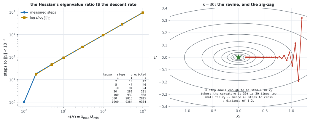
What the eigenvalue RATIO costs gradient descent
    kappa  measured steps   log(eps) / log((k-1)/(k+1))
        1               1                             1
        2              18                            17
        5              47                            46
       10              94                            94
       30             282                           281
      100             939                           938
      300            2816                          2815
     1000            9384                          9384
  The count is linear in kappa, and the closed-form rate predicts it to within
  one step across three orders of magnitude. Newton needs exactly 1 step for
  every one of these, because for a quadratic the second-order model is f.

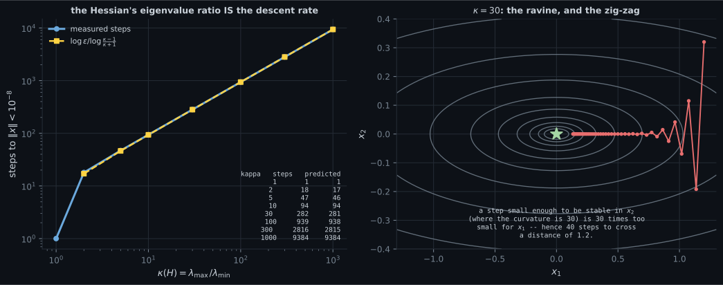
The err / prev^2 column is the whole argument for second-order methods. It settles at about $0.84$ and stays there, which means each error is a constant times the square of the last: $1.08\text{e-}01$, then $9.8\text{e-}03$, then $8.1\text{e-}05$, then $5.5\text{e-}09$. Roughly doubling the number of correct digits per step. Gradient descent’s error falls by a constant factor instead, and the factor is $(\kappa-1)/(\kappa+1)$ — which is why the last table’s step count is linear in the eigenvalue ratio.

And the two facts §5.7’s Remark and Chapter 7 leave you to discover:

curvature_in_the_large.py

import numpy as np
 
 
def hessian(f, x, h=1e-4):
    x = np.asarray(x, dtype=float)
    n = x.size
    H = np.zeros((n, n))
    f0 = f(x)
    for i in range(n):
        ei = np.zeros(n)
        ei[i] = h
        H[i, i] = (f(x + ei) - 2 * f0 + f(x - ei)) / h ** 2
        for j in range(n):
            if i == j:
                continue
            ej = np.zeros(n)
            ej[j] = h
            H[i, j] = (f(x + ei + ej) - f(x + ei - ej)
                       - f(x - ei + ej) + f(x - ei - ej)) / (4 * h ** 2)
    return H
 
 
print("The Remark: for a vector field the Hessian is an (m x n x n) tensor")
F = lambda v: np.array([v[0] ** 2 * v[1], np.sin(v[0]) + v[1] ** 3, v[0] * v[1]])
x0 = np.array([0.7, -0.4])
m, n = 3, 2
T = np.stack([hessian(lambda v, k=k: F(v)[k], x0) for k in range(m)])
exact = np.array([
    [[2 * x0[1], 2 * x0[0]], [2 * x0[0], 0.0]],
    [[-np.sin(x0[0]), 0.0], [0.0, 6 * x0[1]]],
    [[0.0, 1.0], [1.0, 0.0]],
])
print(f"  f : R^{n} -> R^{m}      grad f is {m} x {n}      the Hessian is {T.shape}")
print(f"  one n x n Hessian per output component, stacked")
print(f"  matches the analytic tensor to {np.abs(T - exact).max():.1e}")
print(f"  every n x n slice symmetric to {max(np.abs(T[k] - T[k].T).max() for k in range(m)):.1e}")
print("  There is no 'eigenvalue of a tensor' to read a verdict from -- classification")
print("  is a scalar-output idea, which is why a loss is always a scalar.")
 
print()
print("How rare a minimum is in n dimensions")
print("  Random symmetric Hessians (the Gaussian orthogonal ensemble), 20000 draws each.")
rng = np.random.default_rng(0)
T_DRAWS = 20000
print(f"  {'n':>4}  {'P(all eigenvalues > 0)':>22}  {'coin-flip guess 2^-n':>20}  {'P(saddle)':>10}")
for nd in (1, 2, 3, 4, 5, 6, 8, 10, 12):
    pd = sad = 0
    for _ in range(T_DRAWS):
        M = rng.normal(size=(nd, nd))
        S = (M + M.T) / np.sqrt(2 * nd)
        ev = np.linalg.eigvalsh(S)
        if ev.min() > 0:
            pd += 1
        elif ev.min() < 0 < ev.max():
            sad += 1
    print(f"  {nd:>4}  {pd / T_DRAWS:>22.5f}  {2.0 ** -nd:>20.5f}  {sad / T_DRAWS:>10.5f}")
print("  Note the two middle columns do NOT agree, and the direction matters: the")
print("  coin-flip guess is far too OPTIMISTIC. Eigenvalues of a symmetric matrix")
print("  repel each other rather than landing independently, so all-same-sign is")
print("  rarer than n independent coin flips. By n = 6 it is already unobservable in")
print("  20000 draws -- and a network has millions of parameters.")
 
print()
print("The cheap positive-definiteness test: Cholesky, not eigenvalues")
mats = [("Example 5.7 at (1,1)", np.array([[2.0, 5.0], [5.0, 6.0]])),
        ("bowl", np.array([[2.0, 0.0], [0.0, 4.0]])),
        ("degenerate", np.array([[2.0, 0.0], [0.0, 0.0]])),
        ("ravine", np.array([[1.0, 0.0], [0.0, 30.0]]))]
for name, M in mats:
    try:
        np.linalg.cholesky(M)
        verdict = "succeeds -> positive definite"
    except np.linalg.LinAlgError:
        verdict = "raises LinAlgError -> not positive definite"
    print(f"  {name:22} eigenvalues {np.linalg.eigvalsh(M)}   cholesky {verdict}")
print("  Section 4.3's decomposition exists if and only if H is positive definite, and it")
print("  costs about half an eigendecomposition. If all you need is 'is this a")
print("  minimum', try to factorise and catch the failure.")
 
print()
print("Two routines that are not interchangeable")
H = np.array([[2.0, 5.0], [5.0, 6.0]])
print(f"  eigvals(H)  {np.linalg.eigvals(H)}   dtype {np.linalg.eigvals(H).dtype}")
print(f"  eigvalsh(H) {np.linalg.eigvalsh(H)}   dtype {np.linalg.eigvalsh(H).dtype}   (sorted)")
R = np.array([[0.0, -1.0], [1.0, 0.0]])
print(f"  a NON-symmetric matrix R = {R.tolist()}")
print(f"    eigvals(R)  {np.linalg.eigvals(R)}   -- complex, correctly")
print(f"    eigvalsh(R) {np.linalg.eigvalsh(R)}   -- WRONG, and silent")
print("  eigvalsh reads only the lower triangle and assumes the rest. It does not")
print("  check symmetry, so it will hand you confident nonsense for a matrix that")
print("  is not a Hessian. Use it because Eq 5.146 guarantees symmetry, not by habit.")

output

The Remark: for a vector field the Hessian is an (m x n x n) tensor
  f : R^2 -> R^3      grad f is 3 x 2      the Hessian is (3, 2, 2)
  one n x n Hessian per output component, stacked
  matches the analytic tensor to 1.2e-08
  every n x n slice symmetric to 0.0e+00
  There is no 'eigenvalue of a tensor' to read a verdict from -- classification
  is a scalar-output idea, which is why a loss is always a scalar.
 
How rare a minimum is in n dimensions
  Random symmetric Hessians (the Gaussian orthogonal ensemble), 20000 draws each.
     n  P(all eigenvalues > 0)  coin-flip guess 2^-n   P(saddle)
     1                 0.49800               0.50000     0.00000
     2                 0.14500               0.25000     0.70775
     3                 0.02715               0.12500     0.94745
     4                 0.00240               0.06250     0.99555
     5                 0.00005               0.03125     0.99990
     6                 0.00000               0.01562     1.00000
     8                 0.00000               0.00391     1.00000
    10                 0.00000               0.00098     1.00000
    12                 0.00000               0.00024     1.00000
  Note the two middle columns do NOT agree, and the direction matters: the
  coin-flip guess is far too OPTIMISTIC. Eigenvalues of a symmetric matrix
  repel each other rather than landing independently, so all-same-sign is
  rarer than n independent coin flips. By n = 6 it is already unobservable in
  20000 draws -- and a network has millions of parameters.
 
The cheap positive-definiteness test: Cholesky, not eigenvalues
  Example 5.7 at (1,1)   eigenvalues [-1.38516481  9.38516481]   cholesky raises LinAlgError -> not positive definite
  bowl                   eigenvalues [2. 4.]   cholesky succeeds -> positive definite
  degenerate             eigenvalues [0. 2.]   cholesky raises LinAlgError -> not positive definite
  ravine                 eigenvalues [ 1. 30.]   cholesky succeeds -> positive definite
  Section 4.3's decomposition exists if and only if H is positive definite, and it
  costs about half an eigendecomposition. If all you need is 'is this a
  minimum', try to factorise and catch the failure.
 
Two routines that are not interchangeable
  eigvals(H)  [-1.38516481  9.38516481]   dtype float64
  eigvalsh(H) [-1.38516481  9.38516481]   dtype float64   (sorted)
  a NON-symmetric matrix R = [[0.0, -1.0], [1.0, 0.0]]
    eigvals(R)  [0.+1.j 0.-1.j]   -- complex, correctly
    eigvalsh(R) [-1.  1.]   -- WRONG, and silent
  eigvalsh reads only the lower triangle and assumes the rest. It does not
  check symmetry, so it will hand you confident nonsense for a matrix that
  is not a Hessian. Use it because Eq 5.146 guarantees symmetry, not by habit.

On real data

figure Four critical points, one classifier — and the one it cannot classify matplotlib

The first three are the textbook trio and the eigenvalue signs settle them: [+2.000, +4.000] with 4000 samples up and 0 down; [-4.000, -2.000] the mirror image; [-2.000, +2.000] with 1970 up and 2030 down. The fourth is x1 squared plus x2 to the fourth, whose eigenvalues are [+0.000, +2.000] — the test is silent, and yet all 4000 samples go up, because the origin IS a strict minimum. A zero eigenvalue means ask a higher derivative.

figure Equation 5.146, and the function that ignores it matplotlib

On the left a smooth function, measured over 13 step sizes and 81 grid points: the worst gap is 0.0e+00, exactly, because the five-point stencil computes both orders from the same four corner values and is therefore symmetric by construction. On the right the counterexample xy(x squared minus y squared) over (x squared plus y squared), where the two iterated limits at the origin are -1 and +1 — a gap of exactly 2, at every step size. Equation 5.146 needs its continuity hypothesis.

figure The eigenvalue ratio is the price, in iterations matplotlib

Left: steps to reach 1e-8, against the condition number. Measured 18, 47, 94, 282, 939, 2816, 9384 for kappa of 2, 5, 10, 30, 100, 300, 1000 — and the closed-form rate log(eps)/log((k-1)/(k+1)) predicts 17, 46, 94, 281, 938, 2815, 9384. Right: why. A step small enough to be stable in the steep direction is kappa times too small in the shallow one, so the path crosses the valley instead of running down it. Newton needs one step for every one of these.

Reading the plot

From the four-panel figure. Compare the first and fourth panels. Both have all-non-negative eigenvalues, both have every sample going up, and both are strict minima. But the first panel’s verdict is earned — the eigenvalues are $+2$ and $+4$, positive definite, and the theorem applies. The fourth panel’s is a coincidence: the test could not decide, the sampling found the answer, and if the fourth-order term had been $-x_2^4$ instead the eigenvalues would have been identical and the answer different. The lesson is not “the test usually works”, it is that a zero eigenvalue takes the question out of the Hessian’s hands.

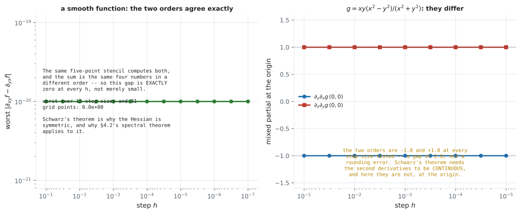
From the middle figure. The left panel is the one to be suspicious of. A measured gap of exactly 0.0e+00, at thirteen step sizes and eighty-one points, is too clean to be a measurement of the function — and it is not one. It is a measurement of the stencil: rearranging $f_{++} - f_{+-} - f_{-+} + f_{--}$ is the same four floating-point numbers in a different order. The right panel is the real test, and it needed a completely different construction — two separate iterated limits with independent inner and outer step sizes — to see anything at all.

From the conditioning figure. The measured and predicted curves lie on top of each other across three orders of magnitude, and that agreement is what licenses the interpretation. The step count is not vaguely related to conditioning; it is $\log \varepsilon / \log\frac{\kappa-1}{\kappa+1}$, to within one step. The right-hand panel shows the mechanism: the largest stable step is set by $\lambda_{\max}$ and the distance to be covered is set by $\lambda_{\min}$, so the two requirements fight, and $\kappa$ is the score.

Pitfalls

Never compare an eigenvalue to zero

A second difference has a truncation floor. For $x_1^2 + x_2^4$ the exact $\partial^2 f/\partial x_2^2$ at the origin is $0$, and the stencil returns $2h^2$ — measured as $2.0\text{e-}04$ at $h = 10^{-2}$ down to $2.0\text{e-}14$ at $h = 10^{-7}$, and positive at every one of them. ev.min() > 0 reports True for a singular Hessian at every step size. Use a tolerance scaled to the size of the entries, and treat “near zero” as the test does not apply.

A symmetric stencil cannot verify Equation 5.146

The five-point mixed stencil builds both $\partial_{xy}f$ and $\partial_{yx}f$ from the same four corner values, so their difference is 0.0e+00 — for every function, including the ones that violate Equation 5.146. If you “check Schwarz’s theorem numerically” this way you have checked nothing. Seeing the failure requires two independent iterated limits, which is what the counterexample table does with an inner step of $10^{-5}$ times the outer one.

Newton’s method finds critical points, not minima

The update $\mathbf{x} - H^{-1}\nabla f$ solves $\nabla f = \mathbf{0}$ and has no preference among solutions. On $f = x_1^2 - x_2^2$ one step lands exactly on the saddle — measured 0.0e+0 — and reports convergence. And where $H$ is indefinite, $-H^{-1}\nabla f$ need not even point downhill: on Example 5.7’s surface at $(2.2, 1.9)$ the Hessian’s eigenvalues are $-4.139$ and $33.02$, and the Newton step lands $0.798$ from the reference point against the gradient step’s $0.740$. This is what trust regions and Hessian modification exist to fix.

eigvalsh does not check that its argument is symmetric

It reads the lower triangle and assumes the rest. Hand it the rotation matrix $\begin{bmatrix} 0 & -1 \\ 1 & 0 \end{bmatrix}$ and it returns $[-1, +1]$ — confident, silent, and wrong; eigvals correctly returns $\pm i$. Use eigvalsh on a Hessian because Equation 5.146 guarantees the symmetry, not because it is the routine you happen to reach for. If $H$ came from an approximation that might not be symmetric, symmetrise it explicitly first with $\tfrac{1}{2}(H + H^\top)$.

The Hessian costs a factor of n more than the gradient

Reverse-mode AD gives you a gradient for about the cost of one function evaluation, and that is what makes first-order training possible. A full Hessian is $n$ gradient-like sweeps, and the linear solve is another $O(n^3)$. At a million parameters the Hessian has $10^{12}$ entries. This is why practical second-order methods never form it: L-BFGS keeps a low-rank approximation from past gradients, Adam keeps only the diagonal, and Hessian-vector products get $H\mathbf{v}$ for one extra sweep without ever building $H$.

In high dimensions a critical point is almost never an optimum

An optimum needs all $n$ eigenvalue signs to agree. Measured on random symmetric matrices: the probability of all-positive is $0.498$ at $n = 1$, $0.145$ at $n = 2$, $0.0272$ at $n = 3$, $0.0024$ at $n = 4$, and by $n = 6$ it does not appear in 20 000 draws. Note the naive $2^{-n}$ coin-flip estimate ($0.125$ at $n = 3$) is far too optimistic: eigenvalues of a symmetric matrix repel, so all-same-sign is rarer than independent flips would suggest. In a million-parameter loss surface, essentially every critical point is a saddle.

Compare

	Gradient, $\nabla f$	Hessian, $H$	Full Taylor series
Shape	$1 \times n$ (Eq 5.40)	$n \times n$ (Eq 5.147)	a tensor per order
Answers	which way, how steeply	what shape, how fast the slope changes	everything, locally
Cost by AD	~1 function evaluation	~$n$ sweeps, plus $O(n^3)$ to solve	grows with the order
At a critical point	says nothing	classifies, unless singular	resolves the singular case
In ML	every training step	L-BFGS, Adam’s diagonal, Laplace approximation	rarely past order 2

Method	Uses	Steps on the convex test	Learning rate?	Fails when
Gradient descent	$\nabla f$	426 (and 3 of 4 rates diverged)	must be tuned	$\kappa$ is large
Newton	$\nabla f$, $H$	8	none needed	$H$ singular or indefinite
Quasi-Newton (L-BFGS)	$\nabla f$ history	between the two	line search	memory, non-smoothness
Adam	$\nabla f$, diagonal moments	between the two	tuned, but forgiving	badly coupled curvature

pch.quizTag Check your understanding

1. What does "the Hessian measures the curvature of the function locally" mean as an equation?

   A The Hessian's trace is the total curvature B The second derivative of f along a unit direction d is exactly d-transpose H d, and over all unit d that quadratic form is squeezed between the smallest and largest eigenvalues of H, attaining both along the eigenvectors C The Hessian's determinant measures how curved the surface is D Curvature is the norm of the Hessian
   pch.quizShowAnswer

   B — The second derivative of f along a unit direction d is exactly d-transpose H d, and over all unit d that quadratic form is squeezed between the smallest and largest eigenvalues of H, attaining both along the eigenvectors — That is why two eigenvalues determine the curvature in infinitely many directions, and why §4.2's spectral theorem is the tool that makes the second-order test work. Measured in the lab above: d-transpose H d agrees with a directly measured second difference to about 1e-15 in all 360 directions.

2. The functions x1^2 + x2^4, x1^2 + x2^3 and x1^2 - x2^4 all have gradient zero and Hessian [[2,0],[0,0]] at the origin. What follows?

   A All three have a minimum at the origin B The origin is a strict minimum for the first and not an optimum for the other two, so no second-order test can distinguish them — the information is not in the Hessian C The Hessian computation must be wrong for at least one of them D They are all saddle points because the Hessian is singular
   pch.quizShowAnswer

   B — The origin is a strict minimum for the first and not an optimum for the other two, so no second-order test can distinguish them — the information is not in the Hessian — A singular Hessian is not a hard case that needs a better tolerance; it is a case the second-order test does not address. The quartic and cubic terms decide, and only a higher-order expansion can see them.

3. Measuring the two mixed partials of a smooth function with the standard five-point stencil gives a gap of exactly 0.0e+00 at 13 step sizes and 81 grid points. What has that established?

   A That Equation 5.146 holds for this function B Almost nothing: the stencil computes both orders from the same four corner values, so its gap is exactly zero for every function, including ones that violate Equation 5.146 C That the function is twice continuously differentiable D That the step size was chosen well
   pch.quizShowAnswer

   B — Almost nothing: the stencil computes both orders from the same four corner values, so its gap is exactly zero for every function, including ones that violate Equation 5.146 — It is a measurement of the stencil, not of the function. To see Equation 5.146 fail you need two separate iterated limits — which on xy(x^2-y^2)/(x^2+y^2) return -1 and +1, a gap of exactly 2 at every step size.

4. On the convex test problem, Newton reached 1e-10 in 8 steps while gradient descent needed 426 and diverged at three of four step sizes. Does that make Newton the better method?

   A Yes, second-order information is strictly better B No. It costs an n-by-n solve per step, so it is impractical at scale, and it solves grad f = 0 rather than seeking a minimum — on x1^2 - x2^2 one step lands exactly on the saddle and reports success C No, because Newton needs a learning rate too D Yes, and the cost is the same
   pch.quizShowAnswer

   B — No. It costs an n-by-n solve per step, so it is impractical at scale, and it solves grad f = 0 rather than seeking a minimum — on x1^2 - x2^2 one step lands exactly on the saddle and reports success — Both halves matter. The cost is why L-BFGS and Adam exist; the wrong-problem issue is why trust regions and Hessian modification exist. A method that converges faster to the wrong kind of point is not automatically an improvement.

5. A random symmetric 3x3 Hessian was positive definite in 2.7% of 20000 draws, against a coin-flip estimate of 2^-3 = 12.5%. What does the discrepancy tell you?

   A The sample size was too small B The eigenvalue signs are not independent — eigenvalues of a symmetric matrix repel — so all-same-sign is RARER than independent flips predict, and the naive estimate is too optimistic C The random matrices were not really symmetric D Nothing, 2.7% and 12.5% are the same order of magnitude
   pch.quizShowAnswer

   B — The eigenvalue signs are not independent — eigenvalues of a symmetric matrix repel — so all-same-sign is RARER than independent flips predict, and the naive estimate is too optimistic — The direction of the error is the point. Even the pessimistic-looking 2^-n understates how rare optima are among critical points, and by n = 6 positive definiteness did not occur once in 20000 draws. In a million-parameter loss surface essentially every critical point is a saddle.

🧪 Try It Yourself

Exercise 1 – Assemble a Hessian by hand

pch.exerciseTag pch.exerciseTitle

Exercise 2 – Curvature along a direction

pch.exerciseTag pch.exerciseTitle

Exercise 3 – Classify, with a tolerance

pch.exerciseTag pch.exerciseTitle

Exercise 4 – One Newton step on a quadratic

pch.exerciseTag pch.exerciseTitle

Exercise 5 – Find the case the test cannot see

pch.exerciseTag pch.exerciseTitle

Recall card

• Higher-order partials read right to left. In Equation 5.146’s notation the operator closest to f acts first, so d2f/dy dx means x first, then y.
• Equation 5.146 needs its hypothesis. Mixed partials commute for a TWICE CONTINUOUSLY differentiable f. On xy(x^2-y^2)/(x^2+y^2) at the origin they exist and differ by exactly 2, measured at every step size.
• Equation 5.147’s Hessian is symmetric, which is why §4.2 applies to it: real eigenvalues and an orthonormal eigenbasis, with no complex arithmetic anywhere.
• “The Hessian measures curvature” means d-transpose H d. The second derivative along a unit direction d is that quadratic form, squeezed between the smallest and largest eigenvalues and attaining both along the eigenvectors. Measured against direct second differences in 360 directions: agreement to about 1e-15.
• The second-order test has FOUR outcomes, not three. All eigenvalues positive, all negative, mixed — and some zero, where it says nothing.
• Three functions, one Hessian, three answers. x1^2 + x2^4 is a strict minimum, x1^2 + x2^3 and x1^2 - x2^4 are not optima, and all three have H = [[2,0],[0,0]] at the origin. A zero eigenvalue means ask a higher derivative, not no optimum.
• Never test an eigenvalue against zero. A second difference’s truncation floor is 2h^2 and it is POSITIVE, so a singular Hessian measures as positive definite at every step size — 2.0e-04 at h = 1e-2 down to 2.0e-14 at h = 1e-7.
• A symmetric stencil cannot verify symmetry. The five-point mixed stencil regroups the same four corner values, so its gap is 0.0e+00 for every function including the counterexamples. Two independent iterated limits are needed to see a failure.
• Newton’s method solves grad f = 0, not “find a minimum”. On x1^2 - x2^2 one step lands exactly on the saddle and reports success; at an indefinite point -H-inverse-grad need not even point downhill.
• Newton converges quadratically and has no learning rate. Measured on a convex problem: 8 steps against gradient descent’s 426, with the error ratio settling at 0.84 times the previous error SQUARED — and three of the four step sizes tried for gradient descent diverged.
• The eigenvalue ratio is the price gradient descent pays. Steps to 1e-8 measured as 18, 94, 939, 9384 for kappa of 2, 10, 100, 1000, matching log(eps)/log((k-1)/(k+1)) to within one step.
• The Hessian costs a factor of n more than the gradient, plus O(n^3) to solve, which is why L-BFGS keeps a low-rank approximation, Adam keeps the diagonal, and Hessian-vector products avoid forming H at all.
• In high dimensions a critical point is almost never an optimum. P(positive definite) measured at 0.498, 0.145, 0.0272, 0.0024 for n = 1 to 4, and unobservable in 20000 draws by n = 6 — rarer than the naive 2^-n guess, because eigenvalues repel.
• Use eigvalsh because Equation 5.146 guarantees symmetry, not by habit. It reads only the lower triangle and does not check; on a rotation matrix it returns a confident, silent, wrong answer.
• For a vector field the Hessian is an (m x n x n) tensor — one n-by-n Hessian per output, each symmetric. There is no eigenvalue of a tensor to classify with, which is one concrete reason a loss is always a scalar.

Next: Linearization and Multivariate Taylor Series — where the gradient and the Hessian turn out to be the first two terms of one series, and the degenerate cases on this page finally get resolved by the third.