Differentiation of Univariate Functions

Chapter 4 asked what is inside a matrix. This chapter asks how a function changes, and it starts where every calculus course starts — one input, one output — because everything later is that idea with more indices.

There are two things on this page. The derivative as the limit of a difference quotient, which you have met; and the Taylor series, which turns a function into a polynomial you can differentiate, integrate and reason about. The second is the one that does the work in the rest of the book: linearisation in §5.8, the Laplace approximation in Chapter 6, and the quadratic models that Chapter 7’s optimisers are built on are all Taylor expansions stopped early.

What you’ll learn

• Definition 5.1 and 5.2: the difference quotient, and the derivative as its limit.
• Why the limit is a definition and not an algorithm — measured, with the exact step size where a finite difference stops improving.
• Definition 5.3: the Taylor polynomial $T_n$, and Definition 5.4: the Taylor series $T_\infty$.
• Why a Taylor polynomial of degree $n$ reproduces a polynomial of degree $n$ exactly, with every later coefficient zero.
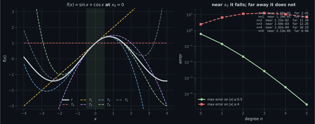
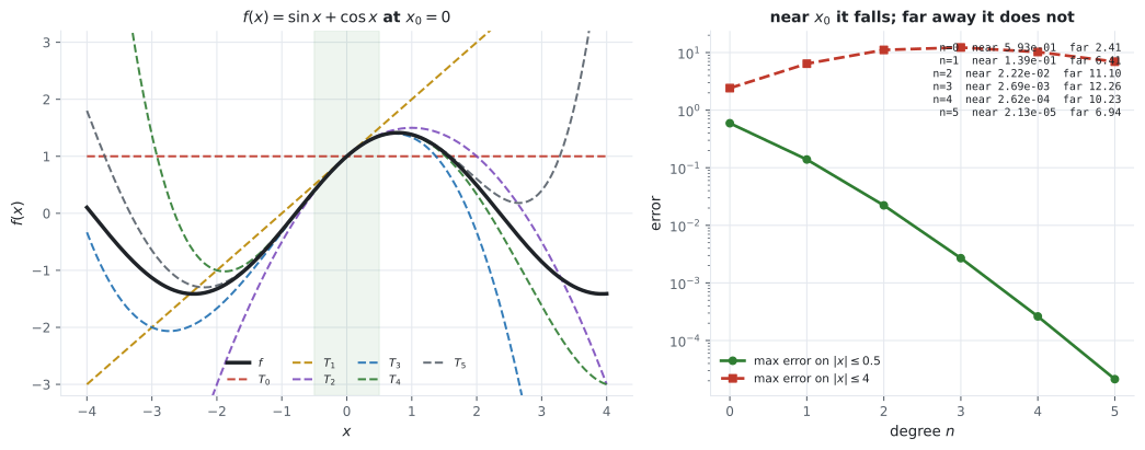
• The thing most treatments skip: near $x_0$ the error falls with degree; far from $x_0$ it grows.
• §5.1.2’s four differentiation rules, and the one that matters most later — the chain rule.

Intuition: a secant that stops moving

Pick a point on a curve and a second point a distance $h$ away. The straight line through them has a slope you can compute from two function values and a division. Now slide the second point towards the first. The secant turns, and — if the function is smooth — it settles on a particular line. Its slope is the derivative.

That is the whole idea, and it is worth noticing what it does not say. It does not say “compute the slope for a small $h$”. It says the slopes converge, and the derivative is the thing they converge to. Those are different claims, and on a computer the difference is the subject of half this page.

diagram Diagram mermaid

  flowchart TD
  DQ["difference quotient
(f(x+h) − f(x)) / h
Def 5.1 — the slope of a secant"]
  DQ -->|"h → 0"| D["derivative f'(x)
Def 5.2 — the slope of the tangent"]
  D --> RULES["§5.1.2 rules
product, quotient, sum, chain"]
  D --> HIGH["f'', f''', … f⁽ᵏ⁾"]
  HIGH --> TP["Taylor polynomial
Tₙ(x) = Σ f⁽ᵏ⁾(x₀)/k! (x−x₀)ᵏ
Def 5.3, Eq 5.7"]
  TP -->|"n → ∞"| TS["Taylor series T∞
Def 5.4, Eq 5.8"]
  TS -->|"x₀ = 0"| MAC["Maclaurin series"]
  TS -->|"f = T∞"| AN["f is analytic"]
  TP --> USE["stop at n = 1: linearisation §5.8
stop at n = 2: the Laplace approximation
and every quadratic model in Ch 7"]
  RULES --> AD["§5.6 automatic differentiation
is the chain rule, applied mechanically"]

The math

The difference quotient and the derivative

Definition 5.1 — Difference Quotient

The difference quotient

$$\frac{\delta y}{\delta x} := \frac{f(x + \delta x) - f(x)}{\delta x} \tag{5.3}$$

computes the slope of the secant line through two points on the graph of $f$.

Definition 5.2 — Derivative

For $h > 0$ the derivative of $f$ at $x$ is defined as the limit

$$\frac{\mathrm{d}f}{\mathrm{d}x} := \lim_{h \to 0}\frac{f(x + h) - f(x)}{h} \tag{5.4}$$

and the secant becomes the tangent.

The book works Example 5.2 — the derivative of $f(x) = x^n$ — straight from Definition 5.2 rather than quoting the power rule, and the point of that exercise is the binomial expansion: every term with $h^{i-1}$ for $i \geq 2$ vanishes in the limit, leaving $\binom{n}{1}x^{n-1} = nx^{n-1}$.

Taylor polynomials

Definition 5.3 — Taylor Polynomial

The Taylor polynomial of degree $n$ of $f: \mathbb{R}\to\mathbb{R}$ at $x_0$ is

$$T_n(x) := \sum_{k=0}^{n}\frac{f^{(k)}(x_0)}{k!}(x - x_0)^k \tag{5.7}$$

where $f^{(k)}(x_0)$ is the $k$-th derivative of $f$ at $x_0$ (assumed to exist) and $\frac{f^{(k)}(x_0)}{k!}$ are the coefficients of the polynomial.

Definition 5.4 — Taylor Series

For a smooth function $f \in C^\infty$, $f:\mathbb{R}\to\mathbb{R}$, the Taylor series of $f$ at $x_0$ is

$$T_\infty(x) = \sum_{k=0}^{\infty}\frac{f^{(k)}(x_0)}{k!}(x-x_0)^k \tag{5.8}$$

For $x_0 = 0$ this is the Maclaurin series. If $f = T_\infty$, then $f$ is called analytic.

The book’s Remark after Definition 5.4 is the one to hold on to: in general, a Taylor polynomial of degree $n$ is an approximation of a function, which does not need to be a polynomial. The Taylor polynomial is similar to $f$ in a neighbourhood around $x_0$. However, a Taylor polynomial of degree $n$ is an exact representation of a polynomial $f$ of degree $\leq n$.

Two words there earn their place. “Neighbourhood” — the guarantee is local, and the measurements below show exactly how local. “Exact” — for a polynomial, $T_n$ is not an approximation at all.

The rules

§5.1.2 lists four, and the chain rule is the one the rest of the chapter is built from:

rule	statement
product	$(fg)' = f'g + fg'$
quotient	$\left(\dfrac{f}{g}\right)' = \dfrac{f'g - fg'}{g^2}$
sum	$(f + g)' = f' + g'$
chain	$\bigl(g(f(x))\bigr)' = g'(f(x))\,f'(x)$

From the book

Section 5.1. Definition 5.1 (Equation 5.3) gives the difference quotient as the slope of a secant, with the remark that for $\delta x < 0$ it is the slope of a secant through the point and one to its left. Definition 5.2 (Equation 5.4) takes the limit. Example 5.2 (Equations 5.5 to 5.6) derives $\mathrm{d}x^n/\mathrm{d}x = nx^{n-1}$ from the definition using the binomial theorem. Section 5.1.1: Definition 5.3 (Equation 5.7) is the Taylor polynomial and Definition 5.4 (Equation 5.8) the Taylor series, with the Maclaurin series as the $x_0 = 0$ case and “analytic” for $f = T_\infty$; the Remark notes that $T_n$ is exact for a polynomial of degree at most $n$. Example 5.3 expands $f(x) = x^4$ at $x_0 = 1$; Example 5.4 expands $f(x) = \sin x + \cos x$ at $x_0 = 0$ and observes the coefficients cycle with period four. Section 5.1.2 lists the product, quotient, sum and chain rules, with Examples 5.5 (product) and the chain-rule worked cases at Equations 5.32 to 5.38.

Worked example by hand

Example 5.3 — x to the fourth, expanded at 1

$f(x) = x^4$, so $f(1) = 1$, $f'(1) = 4$, $f''(1) = 12$, $f'''(1) = 24$, $f^{(4)}(1) = 24$, and $f^{(5)} = 0$ identically. Dividing by $k!$:

$k$	$f^{(k)}(1)$	$k!$	coefficient
0	$1$	$1$	$1$
1	$4$	$1$	$4$
2	$12$	$2$	$6$
3	$24$	$6$	$4$
4	$24$	$24$	$1$
5	$0$	$120$	$0$

$$T_4(x) = 1 + 4(x-1) + 6(x-1)^2 + 4(x-1)^3 + (x-1)^4$$

Those coefficients are $1, 4, 6, 4, 1$ — the fourth row of Pascal’s triangle, which is exactly what the binomial theorem says $\bigl((x-1) + 1\bigr)^4$ should give. So $T_4 = x^4 = f$, and every coefficient past the fourth is zero.

Measured over $[-0.6, 2.6]$: the largest $|f - T_4|$ is $7.11\times10^{-15}$ — machine noise, and it does not change at $T_5$ or $T_6$.

Example 5.4 — sin plus cos, expanded at 0

The derivatives cycle with period four. Since $f^{(k)}(x) = \sin(x + k\pi/2) + \cos(x + k\pi/2)$, at $x = 0$:

$$f^{(k)}(0) = \sin\tfrac{k\pi}{2} + \cos\tfrac{k\pi}{2} = +1, +1, -1, -1, +1, +1, \dots$$

so

$$T_5(x) = 1 + x - \frac{x^2}{2!} - \frac{x^3}{3!} + \frac{x^4}{4!} + \frac{x^5}{5!} = 1 + x - \tfrac{1}{2}x^2 - \tfrac{1}{6}x^3 + \tfrac{1}{24}x^4 + \tfrac{1}{120}x^5$$

This is Exercise 5.4, and it is done.

The error, both ways

Here is the part that is usually left out. Measure $|f - T_n|$ twice: once on a tight interval $|x| \leq 0.5$ around the expansion point, and once on $|x| \leq 4$.

$n$	max error, $\lvert x\rvert \leq 0.5$	max error, $\lvert x\rvert \leq 4$
0	$5.93\times10^{-1}$	$2.41$
1	$1.39\times10^{-1}$	$6.41$
2	$2.22\times10^{-2}$	$11.10$
3	$2.69\times10^{-3}$	$12.26$
4	$2.62\times10^{-4}$	$10.23$
5	$2.13\times10^{-5}$	$6.94$

The left column falls by roughly a factor of ten per degree. The right column rises, more than quadrupling from $n=0$ to $n=3$, before turning around. A Taylor polynomial buys accuracy near a point by giving it up away from it, and any statement that “more terms is better” is missing the qualifier.

See it move

sketch The secant becomes the tangent p5.js Pause Restart

Drag h and watch the secant through (x, f(x)) and (x+h, f(x+h)) rotate onto the tangent. The readout is the slope of the secant against the exact derivative. Drag x to move the point, and note that the convergence is fastest where the curve is straightest.

sketch Taylor polynomials, one degree at a time p5.js Pause Restart

Drag the degree and watch the polynomial wrap itself around the function near x0. The two error readouts are the point: the one measured near x0 falls every time you add a term, the one measured across the whole window does not. Switch functions to see a polynomial become exact.

fieldExample 5.4 and Exercise 5.4, one degree at a timeTaylor polynomials, §5.1.1

T_0(x) = 1

degree 0 of 5|f − T| within ±0.5 6.02e-1on the whole window 2.4142local order h^1

a0 1a1 1a2 -0.5a3 -0.166667a4 0.041667a5 0.008333a6 -0.001389a7 -0.000198

T_n(x0) = f(x0) 0.0e+0

1T_n(x) = sum_{k=0}^{n} f^(k)(x0)/k! * (x - x0)^k      # Eq 5.72 3coeffs = jet(f, x0, N)          # a_k = f^(k)(x0)/k!, by jet arithmetic4for n in 0..N:5    T_n = lambda x: sum(coeffs[k] * (x - x0)**k for k in range(n + 1))6    err = max(abs(f(x) - T_n(x)) for x in window)

degree0|f − T_n| near x06.02e-1on the whole window2.414

Degree 0: T_0 is the constant f(x0) = 1 — a horizontal line touching f at exactly one point. error within ±0.5 of x0 is 6.02e-1.

Play‹›1/6⟲

The coefficients cycle +1, +1, −1, −1. Each frame reports the local order of the error, derived from the first nonzero coefficient not yet used rather than assumed to be n+1.

fieldExample 5.3: a polynomial, expanded at x₀ = 1Taylor polynomials, §5.1.1

T_0(x) = 1

degree 0 of 6|f − T| within ±0.27 1.57e+0on the whole window 44.6976local order h^1

a0 1a1 4a2 6a3 4a4 1a5 0a6 0a7 0a8 0

T_n(x0) = f(x0) 0.0e+0coefficients past degree 4 all zero

1T_n(x) = sum_{k=0}^{n} f^(k)(x0)/k! * (x - x0)^k      # Eq 5.72 3coeffs = jet(f, x0, N)          # a_k = f^(k)(x0)/k!, by jet arithmetic4for n in 0..N:5    T_n = lambda x: sum(coeffs[k] * (x - x0)**k for k in range(n + 1))6    err = max(abs(f(x) - T_n(x)) for x in window)

degree0|f − T_n| near x01.57e+0on the whole window44.70

Degree 0: T_0 is the constant f(x0) = 1 — a horizontal line touching f at exactly one point. error within ±0.26666666666666666 of x0 is 1.57e+0.

Play‹›1/7⟲

Watch degree 4. The error drops to machine noise and the last two frames change nothing, because every remaining coefficient is exactly zero.

From scratch

The obvious way to get $f^{(k)}(x_0)$ numerically is to difference $k$ times. It does not work, and the reason is worth seeing.

taylor_from_scratch.py

import math
import numpy as np
 
def coeffs_by_differencing(f, x0, K, h=1e-3):
    """Repeated central differences. Loses about 8 digits per order."""
    out = []
    for k in range(K + 1):
        # The k-th central difference, from the binomial stencil.
        acc = 0.0
        for j in range(k + 1):
            acc += (-1) ** j * math.comb(k, j) * f(x0 + (k / 2 - j) * h)
        out.append(acc / h ** k / math.factorial(k))
    return out
 
def coeffs_by_jet(x0, K):
    """Truncated-Taylor arithmetic for sin(x) + cos(x): exact at every order."""
    s = [0.0] * (K + 1)
    c = [0.0] * (K + 1)
    s[0], c[0] = math.sin(x0), math.cos(x0)
    u = [0.0] * (K + 1)
    u[0], u[1] = x0, 1.0
    for k in range(1, K + 1):
        ss = sum(j * u[j] * c[k - j] for j in range(1, k + 1))
        cc = sum(j * u[j] * s[k - j] for j in range(1, k + 1))
        s[k], c[k] = ss / k, -cc / k
    return [s[k] + c[k] for k in range(K + 1)]
 
K = 8
exact = [(math.sin(k * math.pi / 2) + math.cos(k * math.pi / 2)) / math.factorial(k)
         for k in range(K + 1)]
diff = coeffs_by_differencing(lambda x: math.sin(x) + math.cos(x), 0.0, K)
jet = coeffs_by_jet(0.0, K)
 
print(f"{'k':>2}  {'exact':>14}  {'by differencing':>16}  {'error':>10}  {'by jet':>14}  {'error':>10}")
for k in range(K + 1):
    print(f"{k:>2}  {exact[k]:>14.10f}  {diff[k]:>16.10f}  {abs(diff[k]-exact[k]):>10.1e}"
          f"  {jet[k]:>14.10f}  {abs(jet[k]-exact[k]):>10.1e}")

output

 k           exact   by differencing       error          by jet       error
 0    1.0000000000      1.0000000000     0.0e+00    1.0000000000     0.0e+00
 1    1.0000000000      0.9999999583     4.2e-08    1.0000000000     0.0e+00
 2   -0.5000000000     -0.4999999583     4.2e-08   -0.5000000000     5.6e-17
 3   -0.1666666667     -0.1666666805     1.4e-08   -0.1666666667     5.6e-17
 4    0.0416666667      0.0416426153     2.4e-05    0.0416666667     6.9e-18
 5    0.0083333333      0.0138777878     5.5e-03    0.0083333333     1.7e-18
 6   -0.0013888889      5.5511151231     5.6e+00   -0.0013888889     4.3e-19
 7   -0.0001984127  -1299.6658423191     1.3e+03   -0.0001984127     8.1e-20
 8    0.0000248016  -225789.4048096796     2.3e+05    0.0000248016     1.0e-20

Read the two error columns, and then read the differencing column itself, because the failure is worse than “inaccurate”.

Differencing holds up to about $k = 4$. Then it does not merely lose precision, it loses the answer:

$k$	true coefficient	by differencing
5	$+0.008333$	$+0.013878$
6	$-0.001389$	$\mathbf{+5.551}$
7	$-0.000198$	$\mathbf{-1299.67}$
8	$+0.0000248$	$\mathbf{-225789.4}$

At $k = 6$ the sign is wrong and the magnitude is out by a factor of four thousand. At $k = 8$ it is out by ten orders of magnitude. This is not an approximation that has degraded; it is noise multiplied by $h^{-8} = 10^{24}$.

The jet column is exact at every order, and the reason is that it never subtracts two nearly equal numbers. Each recurrence is an algebraic identity between coefficients, so the chain rule is applied symbolically and evaluated numerically. That is also, precisely, forward-mode automatic differentiation — which is the connection §5.6 makes explicit.

On real data

figure Definition 5.1 converging to Definition 5.2 matplotlib

Four secants at h = 1.6, 0.8, 0.4 and 0.2, with slopes 1.074466, 1.170422, 1.220578 and 1.239402 against an exact derivative of 1.251610. Each halving of h roughly halves the remaining error — that is what first-order convergence looks like.

figure The half of Definition 5.2 you cannot execute matplotlib

Truncation error falls as h shrinks; round-off error rises. The best forward difference is 2.62e-10 at h = 1.5e-08 and the best central one is 2.88e-13 at h = 2.7e-06. At h = 1e-15 the central estimate is off by 8.07e-02 — 2.8e+11 times worse than its own best.

figure Example 5.4, with the error measured twice matplotlib

Near x0 the error falls by about a factor of ten per degree, from 5.93e-01 at T0 to 2.13e-05 at T5. Across the whole interval it rises from 2.41 to 12.26 by degree 3 before coming back down — the polynomials get better near the centre by getting worse at the edges.

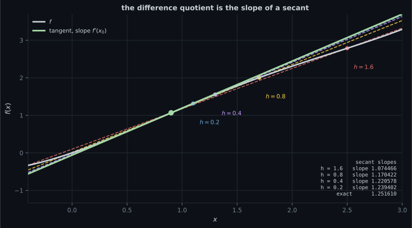
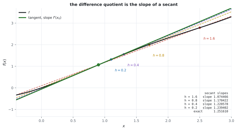
Reading the plot

From the secant figure. The convergence is visible but the rate is the thing to extract. The errors are $0.177$, $0.081$, $0.031$ and $0.012$ for $h = 1.6, 0.8, 0.4, 0.2$ — each roughly half the previous. Halving $h$ halves the error, so the forward difference is first order, and the leading error term is $\frac{h}{2}f''(x)$. That is also why the error is smaller for the same $h$ where the curve is straighter.

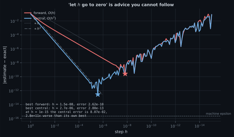
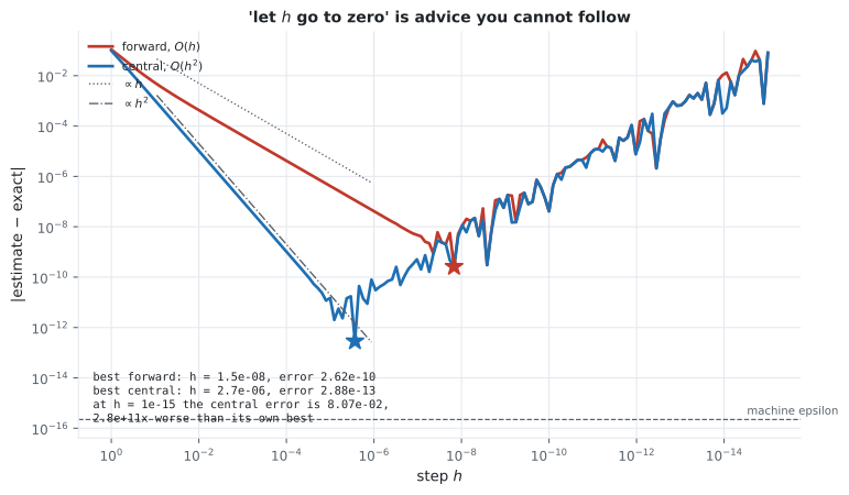
From the round-off figure. This is the figure that changes how you write code.

The forward difference has error $\approx \frac{h}{2}|f''| + \frac{2\varepsilon|f|}{h}$ — truncation falling like $h$, round-off rising like $1/h$. The sum has a minimum, and it is not at the smallest representable $h$:

	best $h$	best error
forward difference	$1.5\times10^{-8}$	$2.62\times10^{-10}$
central difference	$2.7\times10^{-6}$	$2.88\times10^{-13}$

Two consequences. First, $h \approx \sqrt{\varepsilon} \approx 1.5\times10^{-8}$ is the classic forward-difference rule of thumb, and the measurement lands on it. Second, the central difference is not merely better — it is better by three orders of magnitude, for one extra function evaluation. If you are ever going to difference numerically, difference centrally.

And the failure mode is severe: at $h = 10^{-15}$ the central estimate is wrong by $8\times10^{-2}$, which is $2.8\times10^{11}$ times worse than its own best. A gradient check that “uses a really small h to be safe” is not being safe.

From the Taylor figure. The two curves on the right go in opposite directions, and the reason is that a Taylor polynomial is a local object. $T_n$ matches $f$ to order $n$ at $x_0$ and is under no obligation anywhere else — and a degree-$n$ polynomial has to do something as $|x|$ grows, which for $\sin x + \cos x$ (bounded) means running away.

The left column of the table is the guarantee: a factor of about ten per degree on $|x| \leq 0.5$. The right column is the small print.

Pitfalls

Never pick h smaller than about 1e-8 for a forward difference

Measured on this page: the forward difference bottoms out at $h = 1.5\times10^{-8}$ with error $2.6\times10^{-10}$, and by $h = 10^{-15}$ it is wrong by $2.7\times10^{-4}$. The rule of thumb is $h \approx \sqrt{\varepsilon}$ for forward and $h \approx \varepsilon^{1/3} \approx 6\times10^{-6}$ for central, both scaled by the size of $x$. “Smaller is more accurate” is true of the mathematics and false of the arithmetic.

Do not estimate high derivatives by repeated differencing

The from-scratch table above: the 6th coefficient of $\sin x + \cos x$ comes out as $+5.551$ against a true $-0.001389$ — the wrong sign and four thousand times too big — and the 8th as $-225789$ against $+0.0000248$. The $k$-th difference divides by $h^k$, so at $h = 10^{-3}$ and $k = 8$ it multiplies whatever round-off survived by $10^{24}$. Use jet arithmetic, a symbolic derivative, or autodiff — never a tower of finite differences.

More Taylor terms is not uniformly better

For the sigmoid on $[-6, 6]$ the maximum error goes $0.5 \to 1.0 \to 3.5 \to 13 \to 46$ as the degree rises from 0 to 7. Every one of those polynomials is a better approximation near $0$ than the last, and a worse one at the edges. Always state the interval when you quote a Taylor error.

The Taylor series may not converge where you need it

$\log(1+x)$ has a Taylor series at $0$ that converges only for $|x| < 1$, however many terms you take, because of the singularity at $x = -1$. Smoothness at the expansion point tells you nothing about the radius of convergence, which is set by the nearest singularity in the complex plane — which is why $1/(1+x^2)$, a perfectly smooth real function, has a series that diverges beyond $|x| = 1$.

Symmetry hides half the coefficients, and that changes the order

For an odd function about $x_0$, every even coefficient past the constant is zero, so $T_1$ is already accurate to $O(h^3)$ and $T_2$ adds nothing at all. The sigmoid’s local order runs $h^1, h^3, h^3, h^5, h^5, h^7$ as the degree goes $0..5$. Predicting $h^{n+1}$ from the degree alone is wrong for three of the five functions on this page.

Compare

way to get a derivative	exactness	cost	needs
by hand, symbolically	exact	your time	a closed form, and care
forward difference	$O(h)$, floor $\approx 10^{-10}$	1 extra evaluation	nothing
central difference	$O(h^2)$, floor $\approx 10^{-13}$	2 extra evaluations	nothing
jet / forward-mode AD	exact to machine precision	$\approx 2\times$ the function	the code, not the formula
reverse-mode AD (§5.6)	exact to machine precision	$\approx 2.5\times$ the function, all inputs at once	a computation graph
complex-step	$O(h^2)$ with no cancellation	1 complex evaluation	an analytic function

The middle two rows are the ones this page is about. The bottom three are §5.6, and the reason the chapter goes there.

pch.quizTag Check your understanding

1. Definition 5.2 says the derivative is the limit of the difference quotient. Why can that not be executed directly in floating point?

   A Because limits are not computable B Because the truncation error falls like h while the round-off error from subtracting two nearly equal numbers rises like 1/h, so the total has a minimum at a specific h — measured here at 1.5e-08 for a forward difference C Because f(x+h) cannot be evaluated for small h D Because the derivative may not exist
   pch.quizShowAnswer

   B — Because the truncation error falls like h while the round-off error from subtracting two nearly equal numbers rises like 1/h, so the total has a minimum at a specific h — measured here at 1.5e-08 for a forward difference — At h = 1e-15 the central difference on this page is wrong by 8e-02, which is 2.8e+11 times worse than its own best at h = 2.7e-06. Making h smaller past the optimum makes things worse, not better.

2. A central difference costs one extra function evaluation over a forward difference. What does that buy?

   A Nothing measurable B Second-order rather than first-order convergence, and a floor three orders of magnitude lower: 2.9e-13 against 2.6e-10 on this page C The ability to use a smaller h safely D Exactness for all functions
   pch.quizShowAnswer

   B — Second-order rather than first-order convergence, and a floor three orders of magnitude lower: 2.9e-13 against 2.6e-10 on this page — The h-squared error term comes from the odd-order terms cancelling between f(x+h) and f(x-h). It is close to free, so if you are differencing numerically at all, difference centrally.

3. Why is T_4 of x^4 at x0 = 1 not an approximation?

   A It is an approximation, just a very good one B Because a Taylor polynomial of degree n reproduces a polynomial of degree at most n exactly — the coefficients 1, 4, 6, 4, 1 are the binomial expansion of ((x-1)+1)^4, and every coefficient past the fourth is exactly zero C Because x0 = 1 is a special point D Because x^4 is even
   pch.quizShowAnswer

   B — Because a Taylor polynomial of degree n reproduces a polynomial of degree at most n exactly — the coefficients 1, 4, 6, 4, 1 are the binomial expansion of ((x-1)+1)^4, and every coefficient past the fourth is exactly zero — Measured max error over the window: 7.11e-15, unchanged at degrees 5 and 6. The book states this in the Remark after Definition 5.4.

4. Adding Taylor terms drove the sigmoid's maximum error on [-6, 6] from 0.5 up to 46. Is something wrong?

   A Yes, the coefficients must be wrong B No. Each polynomial is strictly better near x0 — the error there falls monotonically — and a Taylor polynomial promises nothing away from the expansion point. A degree-7 polynomial has to grow without bound, and a bounded function does not C Yes, the series diverges D No, but only because the sigmoid is not analytic
   pch.quizShowAnswer

   B — No. Each polynomial is strictly better near x0 — the error there falls monotonically — and a Taylor polynomial promises nothing away from the expansion point. A degree-7 polynomial has to grow without bound, and a bounded function does not — Near x0 the sigmoid's error falls 1.2e-1, 2.5e-3, 2.5e-3, 6.3e-5, ... every added term helps locally. Quoting a Taylor error without naming the interval is the mistake, not the polynomial.

5. The from-scratch table gets the 6th Taylor coefficient as +5.551 instead of -0.001389 using repeated differences, but exactly using jets. What is the difference?

   A The jet uses a smaller step B The jet uses no step at all. Its recurrences are algebraic identities between coefficients, so the chain rule is applied symbolically and only evaluated numerically — nothing nearly-equal is ever subtracted C The jet uses higher precision arithmetic D The jet is an approximation that happens to be closer
   pch.quizShowAnswer

   B — The jet uses no step at all. Its recurrences are algebraic identities between coefficients, so the chain rule is applied symbolically and only evaluated numerically — nothing nearly-equal is ever subtracted — The k-th difference divides by h to the k, so at h = 1e-3 and k = 8 it multiplies surviving round-off by 1e24 — the 8th coefficient came out as -225789 instead of +0.0000248. Jet arithmetic truncated at order 1 is exactly forward-mode automatic differentiation, which is where §5.6 goes.

🧪 Try It Yourself

Exercise 1 – The secant converging, and then not

pch.exerciseTag pch.exerciseTitle

Exercise 2 – Exercises 5.1, 5.2 and 5.3

pch.exerciseTag pch.exerciseTitle

Exercise 3 – Both Taylor errors

pch.exerciseTag pch.exerciseTitle

Exercise 4 – Why repeated differencing fails

pch.exerciseTag pch.exerciseTitle

Exercise 5 – Jets: exact coefficients at every order

pch.exerciseTag pch.exerciseTitle

Recall card

• The difference quotient is the slope of a secant; the derivative is the limit of those slopes, and the limit is a definition rather than an algorithm.
• A forward difference is first order and a central difference second order. Measured: best forward error 2.6e-10 at h = 1.5e-08, best central 2.9e-13 at h = 2.7e-06 — three orders better for one extra function evaluation.
• Making h smaller past the optimum makes things worse. At h = 1e-15 the central estimate is 2.8e+11 times worse than its own best, because subtracting two nearly equal numbers destroys digits.
• The Taylor polynomial of degree n is the sum of f-to-the-k at x0 over k factorial times (x − x0) to the k, and the Taylor series is its limit; at x0 = 0 it is the Maclaurin series, and f = T-infinity means f is analytic.
• For a polynomial of degree at most n, T_n is not an approximation — it is f, with every later coefficient exactly zero. Verified: T_4 of x^4 at x0 = 1 has max error 7.11e-15.
• Near x0 the error falls with degree; on a wide interval it need not. For sin + cos the near error falls 5.9e-1 to 2.1e-5 over six degrees while the far error rises 2.41 to 12.26 and then comes back.
• A Taylor series can fail to converge where the function is perfectly smooth. log(1+x) at 0 converges only for |x| < 1, because the radius is set by the nearest complex singularity.
• Symmetry changes the local order. For an odd function every even coefficient vanishes, so T_1 is already accurate to h-cubed; predicting h-to-the-(n+1) from the degree alone is wrong for most functions.
• Never estimate a high derivative by repeated differencing — the k-th difference divides by h to the k, so the 6th coefficient came out as +5.551 instead of -0.001389 and the 8th as -225789 instead of +0.0000248. Jet arithmetic is exact at every order and is forward-mode autodiff.
• The chain rule is the rule that matters. Everything in §5.2 to §5.6 is the chain rule with more indices.

Next: Partial Differentiation and Gradients — the same definition, one variable at a time.