Eigenvector Computation and Low-Rank Approximations

Pages 1002 and 1004 both ended at the same instruction: take the top $M$ eigenvectors of $\mathbf{S}$. §10.4 is about carrying that out, and it opens two doors:

To get the eigenvalues (and the corresponding eigenvectors) of $\mathbf{S}$, we can follow two approaches: we perform an eigendecomposition and compute the eigenvalues and eigenvectors of $\mathbf{S}$ directly. We use a singular value decomposition.

They give the same answer in exact arithmetic. In floating point they do not, and the difference is measurable.

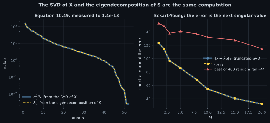
What you’ll learn

• Equations 10.47–10.49: the SVD of $\mathbf{X}$ and the eigendecomposition of $\mathbf{S}$, and $\lambda_d = \sigma_d^2/N$ — measured to $1.4\times10^{-13}$, with the eigenvectors agreeing to $2.1\times10^{-6}$ degrees.
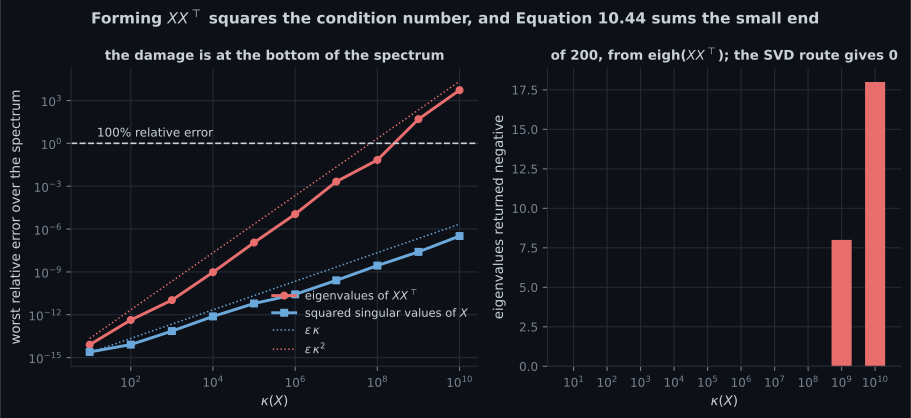
• Why the SVD route is not merely an alternative. Forming $\mathbf{X}\mathbf{X}^\top$ squares the condition number, measured exactly: $\kappa(\mathbf{S})/\kappa(\mathbf{X}) = 246.8358 = \kappa(\mathbf{X})$. At $\kappa(\mathbf{X}) = 10^{10}$ the eigendecomposition returns $18$ negative eigenvalues of $200$ and a worst relative error of $5.3\times10^{3}$; the SVD holds $3.2\times10^{-7}$.
• Equations 10.50–10.51, the Eckart-Young theorem: $\lVert\mathbf{X}-\tilde{\mathbf{X}}_M\rVert_2 = \sigma_{M+1}$ exactly, measured to $7\times10^{-14}$.
• §10.4.2’s Abel-Ruffini note, and what it actually rules out: not eigenvalues, only closed-form roots of the characteristic polynomial past degree $4$.
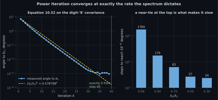
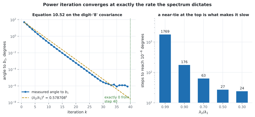
• Equation 10.52, power iteration, with its convergence rate measured against the prediction: $\lambda_2/\lambda_1 = 0.578708$ predicted, $0.578541$ observed by step $25$.
• And what happens when the top of the spectrum is nearly tied: $1769$ steps at a ratio of $0.99$ against $27$ at $0.5$.
• When “wasteful to compute the full decomposition” becomes real: tens of times faster at $D = 2000$ for the top $5$, with eigenvalues agreeing to better than $10^{-10}$.

Intuition: you built a matrix you did not need

$\mathbf{S} = \frac{1}{N}\mathbf{X}\mathbf{X}^\top$ is a summary of $\mathbf{X}$, and forming it is a lossy step. Not lossy in what it represents — the eigenvectors are intact — but in how precisely small quantities survive.

Squaring a number spreads its logarithm. If $\mathbf{X}$‘s singular values span $10^{8}$, then $\mathbf{S}$‘s eigenvalues span $10^{16}$, which is all the room a float64 has. Anything past that is gone, and what is past it is precisely the small end — the end Equation 10.44 sums to get $J_M$.

The SVD reaches the same eigenvectors without ever forming the product. It is not a different method; it is the same method that skips a step which only ever loses information.

diagram Two routes to the same B, and what each costs mermaid

  flowchart LR
  X["X, D x N"] -->|"form X X' / N"| S["S, D x D
kappa squared"]
  S -->|"eigh"| E1["lambda_d, b_d"]
  X -->|"svd, no product formed"| SV["U, Sigma, V'"]
  SV -->|"lambda_d = sigma_d^2 / N"| E2["the same lambda_d, b_d"]
  E1 -.->|"agree to 1.4e-13 here"| E2
  SV --> EY["Eckart-Young:
truncate at M
Equation 10.51"]

§10.4 The two routes

$$\mathbf{S} = \frac{1}{N}\sum_{n=1}^{N}\mathbf{x}_n\mathbf{x}_n^\top = \frac{1}{N}\mathbf{X}\mathbf{X}^\top, \qquad \mathbf{X} = [\mathbf{x}_1,\ldots,\mathbf{x}_N]\in\mathbb{R}^{D\times N} \qquad \text{(10.45), (10.46)}$$

The SVD is $\mathbf{X} = \mathbf{U}\boldsymbol\Sigma\mathbf{V}^\top$ with $\mathbf{U}\in\mathbb{R}^{D\times D}$ and $\mathbf{V}^\top\in\mathbb{R}^{N\times N}$ orthogonal, so

$$\mathbf{S} = \frac{1}{N}\mathbf{U}\boldsymbol\Sigma\underbrace{\mathbf{V}^\top\mathbf{V}}_{=\,\mathbf{I}_N}\boldsymbol\Sigma^\top\mathbf{U}^\top = \frac{1}{N}\mathbf{U}\boldsymbol\Sigma\boldsymbol\Sigma^\top\mathbf{U}^\top \qquad \text{(10.48)}$$

The columns of $\mathbf{U}$ are the eigenvectors of $\mathbf{S}$, and

$$\lambda_d = \frac{\sigma_d^2}{N} \qquad \text{(10.49)}$$

$d$	$\sigma_d$	$\sigma_d^2/N$	$\lambda_d$	gap
$1$	$162.397363$	$151.56841162$	$151.56841162$	$1.1\times10^{-13}$
$2$	$123.540283$	$87.71380214$	$87.71380214$	$1.4\times10^{-14}$
$3$	$114.453400$	$75.28494722$	$75.28494722$	$1.4\times10^{-13}$
$4$	$96.982435$	$54.05513090$	$54.05513090$	$5.0\times10^{-14}$
$5$	$95.498161$	$52.41321109$	$52.41321109$	$2.1\times10^{-14}$

Largest gap over all $64$: $1.4\times10^{-13}$. Worst angle between $\mathbf{u}_d$ and $\mathbf{b}_d$ over the top $20$: $2.1\times10^{-6}$ degrees.

figure Equation 10.49 measured, and Eckart-Young measured matplotlib

Left: the squared singular values divided by N and the eigenvalues of S are one curve. Right: the truncated SVD's spectral-norm error is exactly the next singular value, matching to 7e-14 — while the best of 400 random rank-M subspaces never gets close.

Why this is not a matter of taste

$\kappa(\mathbf{X}\mathbf{X}^\top) = \kappa(\mathbf{X})^2$. Measured on the digit-”8” data:

	value
$\kappa(\mathbf{X})$, from the nonzero singular values	$2.468358\times10^{2}$
$\kappa(\mathbf{S})$, from the nonzero eigenvalues	$6.092792\times10^{4}$
their ratio	$246.8358 = \kappa(\mathbf{X})$

At $\kappa = 247$ that is harmless. Pushed on a synthetic $200\times200$ matrix whose singular values span a chosen range:

$\kappa(\mathbf{X})$	$\kappa(\mathbf{X}\mathbf{X}^\top)$	worst relative error, eigh	worst relative error, SVD	negative eigenvalues from eigh
$10^{2}$	$10^{4}$	$4.3\times10^{-13}$	$8.2\times10^{-15}$	$0$
$10^{4}$	$10^{8}$	$9.5\times10^{-10}$	$7.6\times10^{-13}$	$0$
$10^{6}$	$10^{12}$	$1.1\times10^{-5}$	$2.7\times10^{-11}$	$0$
$10^{8}$	$10^{16}$	$6.9\times10^{-2}$	$2.8\times10^{-9}$	$0$
$10^{10}$	$10^{20}$	$\mathbf{5.3\times10^{3}}$	$\mathbf{3.2\times10^{-7}}$	$\mathbf{18}$ of $200$

figure The red line has twice the slope, which is the whole story matplotlib

The relative error of the eigendecomposition route grows like epsilon times kappa squared; the SVD route like epsilon times kappa. Both reference lines are drawn and both are followed. Past kappa = 1e8 the red line crosses 100 percent relative error, and by 1e10 eighteen of two hundred eigenvalues of a positive semi-definite matrix come back negative.

The large eigenvalues are fine either way; the small ones are the whole point

It is worth being precise about what breaks. At $\kappa(\mathbf{X}) = 10^{9}$, individual eigenvalues:

	true	eigh of $\mathbf{X}\mathbf{X}^\top$	SVD of $\mathbf{X}$
$\lambda_1$	$1.0000\times10^{0}$	$1.0000\times10^{0}$	$1.0000\times10^{0}$
$\lambda_{100}$	$1.1098\times10^{-9}$	$1.1098\times10^{-9}$	$1.1098\times10^{-9}$
$\lambda_{180}$	$6.4424\times10^{-17}$	$6.0118\times10^{-17}$	$6.4424\times10^{-17}$
$\lambda_{200}$	$1.0000\times10^{-18}$	$\mathbf{-4.8565\times10^{-17}}$	$1.0000\times10^{-18}$

If you only want $\mathbf{b}_1,\ldots,\mathbf{b}_M$ for a small $M$, the eigendecomposition of $\mathbf{S}$ is perfectly safe — those eigenvalues are at the top. But $J_M$ is a sum over the small end (Equation 10.44), and so is the reconstruction error you report. Measured at $M = 100$ with $\kappa = 10^{9}$: $J_M$ from eigh carries a relative error of $4.5\times10^{-8}$ against the SVD route’s $3.1\times10^{-13}$.

And a negative eigenvalue of a covariance matrix is not a small error — it is an impossible answer, and one that propagates straight into a variance-explained percentage above $100\%$.

§10.4.1 Eckart-Young

The best rank-$M$ approximation in the spectral norm,

$$\tilde{\mathbf{X}}_M := \operatorname*{arg\,min}_{\mathrm{rk}(\mathbf{A})\leq M}\lVert\mathbf{X}-\mathbf{A}\rVert_2 \qquad \text{(10.50)}$$

is obtained “by truncating the SVD at the top-$M$ singular value”:

$$\tilde{\mathbf{X}}_M = \mathbf{U}_M\boldsymbol\Sigma_M\mathbf{V}_M^\top \in \mathbb{R}^{D\times N} \qquad \text{(10.51)}$$

$M$	$\lVert\mathbf{X}-\tilde{\mathbf{X}}_M\rVert_2$	$\sigma_{M+1}$	gap	best of $3000$ random rank-$M$
$1$	$123.540283$	$123.540283$	$7.1\times10^{-14}$	$148.274427$
$2$	$114.453400$	$114.453400$	$7.1\times10^{-14}$	$145.287326$
$5$	$86.072481$	$86.072481$	$5.7\times10^{-14}$	$136.205379$
$10$	$54.732079$	$54.732079$	$3.6\times10^{-14}$	$121.669733$

The Frobenius-norm version, which is the one PCA actually optimises:

$M$	$\lVert\mathbf{X}-\tilde{\mathbf{X}}_M\rVert_F$	$\sqrt{\sum_{j>M}\sigma_j^2}$
$1$	$320.294771$	$320.294771$
$5$	$236.011581$	$236.011581$
$20$	$101.622901$	$101.622901$

Squaring the last column and dividing by $N$ recovers page 1004’s $J_M$ — $320.294771^2/174 = 589.590460$ — because $\lVert\mathbf{X}-\tilde{\mathbf{X}}_M\rVert_F^2 = \sum_{j>M}\sigma_j^2 = N\sum_{j>M}\lambda_j$. Eckart-Young and Equation 10.44 are the same theorem in two notations.

§10.4.2 Practical aspects

Two claims here, and they are about different things.

Abel-Ruffini. Eigenvalues are roots of the characteristic polynomial, and for degree $5$ or more there is “no algebraic solution” — no formula in radicals. “Therefore, in practice, we solve for eigenvalues or singular values using iterative methods.”

What Abel-Ruffini does and does not forbid

It rules out a closed-form expression in radicals for the roots of a general polynomial of degree $\geq 5$. It says nothing about computing those roots to any accuracy you like — that is routine, and np.linalg.eigh does it in microseconds for a $64\times64$ matrix.

Nor is the characteristic polynomial how anyone computes eigenvalues. Forming it and rooting it is catastrophically ill-conditioned; real implementations use QR iteration on the matrix directly. The theorem explains why the algorithms are iterative rather than a formula, not why they are hard.

Only $M$ vectors are wanted. “It would be wasteful to compute the full decomposition, and then discard all eigenvectors with eigenvalues that are beyond the first few.” Measured, full eigh against a Lanczos solve for the top $5$:

size of $\mathbf{S}$	full eigh	eigsh, $k = 5$	speed-up	top-$5$ eigenvalues agree to
$500\times500$	$55.53$ ms	$2.64$ ms	$21.1\times$	$4.5\times10^{-13}$
$2000\times2000$	$1588.52$ ms	$37.43$ ms	$\mathbf{42.4\times}$	$4.5\times10^{-13}$

One run on one machine — the timings move between runs (a repeat gave $31\times$ and $30\times$), but the shape does not: a full decomposition is cubic in $D$, and five vectors were asked for.

At the chapter’s own $D = 784$ this is already worth having; at the $D = 10{,}000$ of §10.5’s $100\times100$ images it is the difference between feasible and not.

Equation 10.52, and how fast it actually is

$$\mathbf{x}_{k+1} = \frac{\mathbf{S}\mathbf{x}_k}{\lVert\mathbf{S}\mathbf{x}_k\rVert}, \qquad k = 0, 1, \ldots \qquad \text{(10.52)}$$

“This sequence of vectors converges to the eigenvector associated with the largest eigenvalue” — and the rate is not stated, but it is $\lambda_2/\lambda_1$ per step. On the digit-”8” covariance, where that ratio is $0.578708$:

$k$	angle to $\mathbf{b}_1$, degrees	ratio to the previous step
$1$	$4.93\times10^{1}$	—
$2$	$2.62\times10^{1}$	$0.532116$
$5$	$3.40\times10^{0}$	$0.516479$
$10$	$1.60\times10^{-1}$	$0.555946$
$15$	$9.40\times10^{-3}$	$0.572467$
$20$	$5.95\times10^{-4}$	$0.577269$
$25$	$3.84\times10^{-5}$	$\mathbf{0.578541}$

The observed ratio climbs to the predicted $0.578708$ as the contributions from $\lambda_3$ onwards die out faster and only the $\lambda_2$ component is left. The angle reaches exactly $0$ at step $40$.

figure The rate is the eigenvalue gap, and nothing else matplotlib

A straight line on a log scale is geometric convergence. The dashed line is the predicted ratio 0.578708 raised to the k, drawn with no fitting. The right panel is the same fact as a cost: when the top two eigenvalues are nearly tied, the iteration has almost nothing to separate them with.

$\lambda_2/\lambda_1$	steps to reach $10^{-6}$ degrees
$0.99$	$\mathbf{1769}$
$0.90$	$176$
$0.70$	$63$
$0.50$	$27$
$0.30$	$24$

“The original Google PageRank algorithm uses such an algorithm for ranking web pages based on their hyperlinks.” The same table explains why PageRank’s damping factor exists: it is chosen partly to keep the second eigenvalue away from the first.

pch.quizTag Is the computation clear?

1. Why is the SVD of X preferable to the eigendecomposition of S when the small eigenvalues matter?

   A It is faster B Forming X X-transpose squares the condition number, so the relative error on small eigenvalues grows like kappa squared instead of kappa C The SVD gives different eigenvectors D The eigendecomposition does not work on rectangular matrices
   pch.quizShowAnswer

   B — Forming X X-transpose squares the condition number, so the relative error on small eigenvalues grows like kappa squared instead of kappa — Measured on a 200-by-200 matrix: at condition number 1e8 the eigendecomposition route already has 6.9 percent worst relative error, and at 1e10 it has 5.3e+03 and returns 18 negative eigenvalues — an impossible answer for a covariance matrix. The SVD route holds 3.2e-07. J_M sums exactly the small end.

2. What does the Eckart-Young theorem say the spectral-norm error of the truncated SVD is?

   A The sum of the discarded singular values B Exactly sigma_(M+1), the largest singular value you dropped C The square root of M D Zero
   pch.quizShowAnswer

   B — Exactly sigma_(M+1), the largest singular value you dropped — Measured to 7e-14 at M = 1, 2, 5 and 10. In the Frobenius norm the error is the square root of the sum of the squared discarded singular values, which divided by N is exactly page 1004's J_M — 320.294771 squared over 174 is 589.590460. Eckart-Young and Equation 10.44 are one theorem in two notations.

3. What does the Abel-Ruffini theorem actually rule out?

   A Computing eigenvalues of matrices larger than 4 by 4 B A closed-form expression in radicals for the roots of a general polynomial of degree five or more — nothing about computing them numerically C The existence of eigenvalues D Iterative methods
   pch.quizShowAnswer

   B — A closed-form expression in radicals for the roots of a general polynomial of degree five or more — nothing about computing them numerically — It explains why eigenvalue algorithms are iterative rather than a formula. It says nothing about accuracy or difficulty — np.linalg.eigh handles a 64-by-64 matrix in under a millisecond. And nobody computes eigenvalues by rooting the characteristic polynomial anyway; that route is catastrophically ill-conditioned.

4. Power iteration converges at what rate?

   A Always one step B Geometrically, at the ratio of the second eigenvalue to the first C Linearly in the dimension D D It does not converge for symmetric matrices
   pch.quizShowAnswer

   B — Geometrically, at the ratio of the second eigenvalue to the first — On the digit-8 covariance the ratio is 0.578708 and the measured step-to-step ratio reaches 0.578541 by iteration 25, with no fitting. The cost of a near-tie is steep: 1,769 steps at a ratio of 0.99 against 27 at 0.5. That is also why PageRank's damping factor is chosen as it is.

Exercises

Exercise 1 – One decomposition, two names

pch.exerciseTag pch.exerciseTitle

Exercise 2 – What squaring the condition number costs

pch.exerciseTag pch.exerciseTitle

Exercise 3 – Eckart-Young, and its Frobenius twin

pch.exerciseTag pch.exerciseTitle

Exercise 4 – Power iteration, and the rate it converges at

pch.exerciseTag pch.exerciseTitle

Exercise 5 – The cost of computing what you throw away

pch.exerciseTag pch.exerciseTitle

Recall card

• Section 10.4 offers two routes to the same basis: the eigendecomposition of S, or the singular value decomposition of X.
• Equation 10.49 connects them: each eigenvalue is the corresponding squared singular value divided by N, measured to 1.4e-13, with eigenvectors agreeing to two millionths of a degree.
• Forming X X-transpose squares the condition number — measured exactly on the digit data, where the ratio of the two condition numbers is itself the condition number.
• That costs relative accuracy at the bottom of the spectrum, which is exactly what Equation 10.44 sums. At condition number 1e8 the eigendecomposition route has 6.9 percent worst relative error; at 1e10 it has 5.3e+03.
• And it returns 18 negative eigenvalues out of 200 for a positive semi-definite matrix, an impossible answer that flows straight into any variance-explained figure.
• The large eigenvalues are fine either way, so if you only want the top few components, either route is safe.
• Eckart-Young says the truncated SVD is the best rank-M approximation, and its spectral-norm error is exactly the next singular value — measured to 7e-14.
• Its Frobenius error squared, divided by N, is page 1004’s reconstruction error. Eckart-Young and Equation 10.44 are one theorem in two notations.
• Abel-Ruffini rules out a closed-form formula in radicals past degree four, and nothing else. Eigenvalues are still computed to full precision, iteratively, and never by rooting the characteristic polynomial.
• Power iteration converges geometrically at the ratio of the second eigenvalue to the first — predicted 0.578708, measured 0.578541 by step 25, with nothing fitted.
• A near-tie at the top is what makes it slow: 1,769 steps at a ratio of 0.99 against 27 at 0.5. That is also why PageRank has a damping factor.
• Asking for only the top five eigenpairs is tens of times faster at D equal to 2000, and agrees to better than 1e-10.

Next: PCA in High Dimensions — §10.5, where $N \ll D$ and the $D\times D$ covariance matrix is the wrong object to decompose entirely.