Data Augmentation for Small Datasets

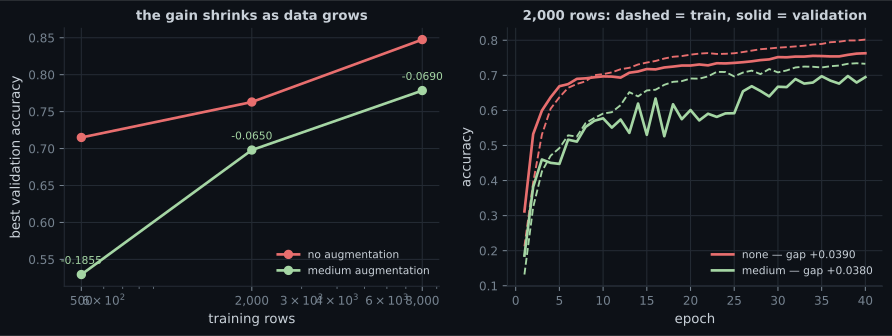
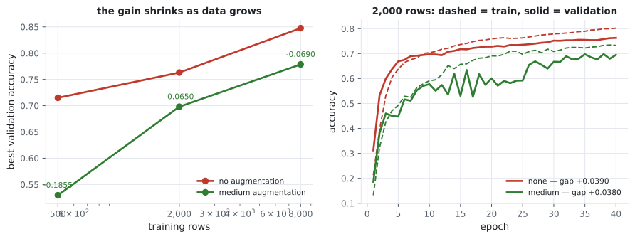
Data augmentation is the standard prescription for a small dataset: rotate, shift and flip your training images to manufacture more of them. On Fashion-MNIST it made every model worse.

Training rows	No augmentation	Medium augmentation	Gain
500	0.7150	0.5295	−0.1855
2,000	0.7630	0.6980	−0.0650
8,000	0.8475	0.7785	−0.0690

That is not a bug, and this page is about why — and about the measurement that shows what augmentation did buy, which turns out to be something else entirely.

What you’ll learn

• Why augmentation is a statement about invariance, and what happens when the statement is false.
• The measurement that redeems it: on rotated test data, augmentation turned 0.5965 into 0.7070.
• Why RandomRotation(0.15) is ±54°, not a mild jitter.
• Why a fixed epoch budget makes augmentation look worse than it is — and how much worse.
• The diagnostic that tells you in advance whether augmentation can help at all.

Augmentation is a claim about your data

Every augmentation encodes an assumption: the label does not change under this transformation. Rotating a boot by 20° should still be a boot, so the model should learn to be invariant to rotation.

That assumption is about the test set, not the training set. Fashion-MNIST images are centred, size-normalised and axis-aligned — every one of them, in training and test. So rotation invariance is not a property the task rewards; it is capacity spent on variation the test set never contains.

The un-augmented model’s train–validation gap says the same thing from another angle:

Rows	Best validation accuracy	Train − validation gap
500	0.7150	0.0285
2,000	0.7630	0.0390
8,000	0.8475	0.0325

A gap of 0.03 is not overfitting. Augmentation is a regulariser, and this model has almost nothing to regularise. Reaching for it here is treating a disease the patient does not have.

figure Fashion-MNIST, 40 epochs matplotlib

Augmentation lost at every size, and lost most at the smallest — the opposite of the usual claim. The right panel shows why the train-validation gap matters: both models track their own training accuracy closely, so neither is memorising, and a regulariser has nothing to fix.

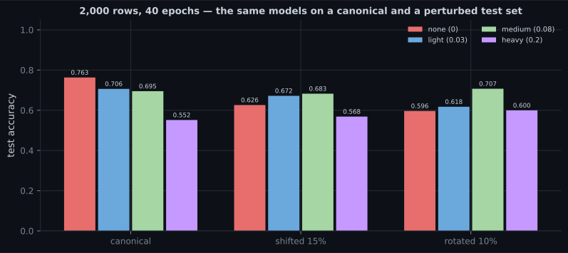
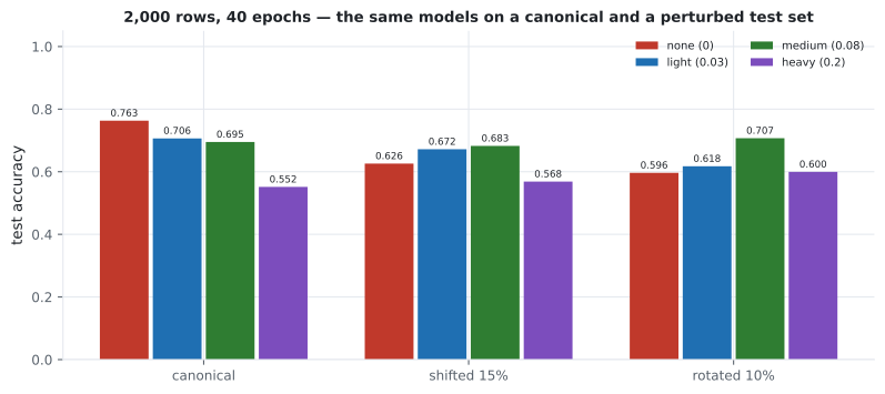
The measurement that changes the verdict

If augmentation buys invariance rather than accuracy, then the way to see it is to test on data that needs the invariance. Same four models, three test sets: the canonical one, one shifted by up to 15%, one rotated by up to 10% of a turn.

Strength	Canonical	Shifted 15%	Rotated 10%	Canonical − shifted
none	0.7630	0.6260	0.5965	0.1370
light (0.03)	0.7065	0.6720	0.6175	0.0345
medium (0.08)	0.6950	0.6825	0.7070	0.0125
heavy (0.20)	0.5515	0.5685	0.5995	−0.0170

figure 2,000 rows, 40 epochs — the same models on three test sets matplotlib

Read the un-augmented bars left to right: 0.763, 0.626, 0.596. That model loses 0.1370 the moment the test images move and 0.1665 when they rotate — it never had to cope with either. The medium-augmented model reads 0.695, 0.683, 0.707: almost flat. It gave up 0.068 on canonical data and bought back 0.1105 on rotated data. Neither model is better; they are optimised for different deployment conditions.

That is the honest statement of what augmentation does:

• It costs accuracy on data drawn from the same distribution as the training set.
• It buys accuracy on data that is not — measured +0.1105 on rotation, +0.0565 on shift.
• The right amount depends entirely on which of those your production data looks like, and nothing in your training set can tell you.

Heavy augmentation (±72° rotation) is bad everywhere, which is its own lesson: an invariance the task genuinely does not have is not free even when the test set is perturbed.

Keras’ rotation factor is in turns

RandomRotation(0.15) is not a small rotation

keras.layers.RandomRotation(0.15)     # +/- 0.15 * 360 = +/- 54 degrees
keras.layers.RandomRotation(0.03)     # +/- 10.8 degrees — this is "light"

The first version of this page used 0.15 as its “medium” setting, on the assumption that it meant something like 15%. It is ±54°, which turns a sandal into an unrecognisable blob. The strengths on this page are 0.03 / 0.08 / 0.20 — ±10.8°, ±28.8° and ±72°.

figure One image through the pipeline eight times matplotlib

Mean absolute pixel change across the eight draws ranged from 0.1360 to 0.1948, and no two draws were identical. Look at the black borders: every shift and rotation pulls the garment away from the frame and pads with zeros, so the model also learns that a border of black is normal — a second, unintended change to the input distribution.

The budget trap

The first version of this experiment ran 15 epochs and concluded that augmentation costs 0.16–0.20 accuracy everywhere. It does not:

Rows	Setup	Best epoch	Accuracy at epoch 15	Best accuracy
500	none	39	0.5780	0.7150
500	medium	40	0.4715	0.5295
2,000	none	40	0.7180	0.7630
2,000	medium	38	0.5305	0.6980
8,000	none	40	0.8075	0.8475
8,000	medium	33	0.7225	0.7785

At 2,000 rows the augmented model reads 0.5305 at epoch 15 and 0.6980 at its best — 0.1675 of the apparent penalty was just an unfinished run. Augmentation makes every epoch a slightly different task, so convergence takes longer by construction. Comparing at a fixed epoch count measures the budget.

diagram Diagram mermaid

  flowchart TB
  A["is the train-validation gap large?"] -->|"no — 0.03 here"| B["augmentation has nothing
to regularise"]
  A -->|"yes"| C["will deployment data
differ in pose?"]
  C -->|"no"| D["augment weakly or not at all"]
  C -->|"yes"| E["augment for that specific variation"]
  E --> F["measure on a perturbed test set,
not just the canonical one"]
  B --> F
  F --> G["train to convergence,
not to a fixed epoch count"]

Which transformations are safe

Transformation	Label-preserving?
RandomFlip("horizontal")	usually — a sneaker mirrored is a sneaker
RandomFlip("vertical")	no for clothing: Fashion-MNIST has no upside-down boots
RandomRotation(small)	yes within a few degrees
RandomZoom, RandomTranslation	yes, but both introduce black borders
horizontal flip on text or digits	no — a mirrored 2 is not a 2

The test is always the same question: would a human give the augmented image the same label? If yes, it is a valid augmentation; if the test set never contains such images, it is a valid augmentation that costs you accuracy.

sketch Invariance you asked for, invariance you needed p5.js Pause Restart

Choose how much the deployment data differs from the training data, and see which model wins. The numbers are the measured ones.

sketch The measured table, ranked p5.js Pause Restart

Click a column to rank every row by it. The bars are that column's values and the highest and lowest are computed from the numbers, not written in.

Pitfalls

• Augmenting a model that is not overfitting. The gap here was 0.03, and augmentation cost up to 0.1855.
• Judging augmentation on the canonical test set alone. It lost 0.068 there and won 0.1105 on rotated data — one number without the other is half the story.
• Comparing at a fixed epoch count. 0.1675 of the apparent penalty at 2,000 rows was an unfinished run.
• Reading Keras’ rotation factor as a percentage. RandomRotation(0.15) is ±54°.
• Using vertical flips on clothing, or horizontal flips on digits and text. The label does not survive.
• Ignoring the borders. Every shift and rotation pads with black, so the model also learns that black borders are normal.
• Assuming more augmentation is safer. Heavy (±72°) was worst on all three test sets, including the perturbed ones.

Recap

• Augmentation lost accuracy at every dataset size on canonical Fashion-MNIST: −0.1855, −0.0650, −0.0690.
• The un-augmented train–validation gap was ~0.03 — there was nothing to regularise.
• On perturbed test data the ranking reverses: rotated 0.5965 → 0.7070, shifted 0.6260 → 0.6825.
• The un-augmented model’s canonical-minus-shifted drop was 0.1370; the medium-augmented model’s was 0.0125.
• RandomRotation(0.15) is ±54°; the settings here are ±10.8°, ±28.8° and ±72°.
• Augmentation delays convergence: at 2,000 rows the augmented model gained 0.1675 after epoch 15.

Next

Augmentation manufactures inputs. The next page stops classifying whole images and starts labelling every pixel: Image Segmentation.

pch.quizTag pch.quizDefaultTitle

1. Augmentation cost 0.1855 accuracy at 500 training rows on Fashion-MNIST. What is the most likely explanation?

   A The augmentation was implemented incorrectly B Fashion-MNIST is centred and pose-normalised in both train and test, so rotation and shift invariance are capacity spent on variation the test set never contains C 500 rows is too many for augmentation to help D Augmentation only works on colour images
   pch.quizShowAnswer

   B — Fashion-MNIST is centred and pose-normalised in both train and test, so rotation and shift invariance are capacity spent on variation the test set never contains — The un-augmented train-validation gap was 0.0285 — the model was not overfitting, so a regulariser had nothing to fix.

2. On rotated test data the augmented model scored 0.7070 against the un-augmented model's 0.5965. What does that establish?

   A Augmentation is better after all B Augmentation buys invariance rather than accuracy — it costs on data drawn from the training distribution and pays on data that is not C The rotated test set is easier D The models should be retrained
   pch.quizShowAnswer

   B — Augmentation buys invariance rather than accuracy — it costs on data drawn from the training distribution and pays on data that is not — The un-augmented model's canonical-minus-shifted drop was 0.1370 against 0.0125 for the augmented one. Which model is 'better' depends entirely on what the deployment data looks like.

3. What does RandomRotation(0.15) do?

   A Rotates by up to 15 degrees B Rotates by up to 0.15 of a full turn — plus or minus 54 degrees, which is enough to make a sandal unrecognisable C Rotates 15% of the images D Rotates by 15 radians
   pch.quizShowAnswer

   B — Rotates by up to 0.15 of a full turn — plus or minus 54 degrees, which is enough to make a sandal unrecognisable — The factor is in turns. The settings on this page are 0.03, 0.08 and 0.20 — plus or minus 10.8, 28.8 and 72 degrees.

4. At 2,000 rows the augmented model scored 0.5305 at epoch 15 and 0.6980 at its best. What does that mean for benchmarking?

   A Augmented models are unstable B Augmentation makes each epoch a slightly different task, so it converges later — comparing at a fixed epoch count measures the budget, not the treatment C The learning rate was too low D Fifteen epochs is enough for any model
   pch.quizShowAnswer

   B — Augmentation makes each epoch a slightly different task, so it converges later — comparing at a fixed epoch count measures the budget, not the treatment — 0.1675 of the apparent penalty was simply an unfinished run. Report the best epoch, or train both to convergence.

5. Which diagnostic tells you in advance whether augmentation is likely to help?

   A The number of training rows B The train-validation gap plus knowledge of how the deployment data differs from the training data — augmentation regularises, and it only pays for invariances the test data actually needs C The model's parameter count D The learning rate
   pch.quizShowAnswer

   B — The train-validation gap plus knowledge of how the deployment data differs from the training data — augmentation regularises, and it only pays for invariances the test data actually needs — A gap of 0.03 says there is nothing to regularise; the deployment question says whether the invariance is worth buying anyway.

🧪 Try It Yourself

pch.exerciseTag pch.exerciseTitle

pch.exerciseTag pch.exerciseTitle

pch.exerciseTag pch.exerciseTitle

pch.exerciseTag pch.exerciseTitle

pch.exerciseTag pch.exerciseTitle