Sentiment Analysis Tutorial

This is the phase’s bake-off. Five model families, one dataset, one split, one budget — so the comparison means something. The families are the ones the last four pages built, in the order they were introduced.

The simplest one wins.

Family	Parameters	Test accuracy	Seconds
TF-IDF + logistic regression	9,768	0.8632	8.4
average embedding	320,033	0.8575	36.6
1D convolution	330,369	0.8495	83.1
transformer block	328,577	0.8462	460.2
LSTM	328,353	0.8415	263.1

A linear model over word counts beat a transformer by 0.0170 while training 55× faster and using 34× fewer parameters. This page is about why, and about what would have to change for the ordering to flip.

What you’ll learn

Why the reading order of this phase is not the ranking of its models.
What each family costs in wall-clock, and where that cost goes.
How the ranking changes with dataset size — the gap is largest at 1,000 rows.
Whether the winning model’s confidence means anything (it does, measured).
The checks that make a text-classification result trustworthy.

The bake-off

Two panels. Left: horizontal bars of test accuracy for five families, all between 0.8415 and 0.8632, each annotated with its parameter count — TF-IDF plus logistic leads with only 9,768 parameters. Right: accuracy against training seconds on a log axis, with TF-IDF in the top-left corner at 8.4 seconds and the transformer at the far right at 460 seconds and lower accuracy. — The right panel is the one to keep. Every neural family sits below and to the right of the bag-of-words baseline: more time, less accuracy. The spread in accuracy is 0.0217 across all five families — smaller than the difference a weighting change made on the TF-IDF page — while the spread in cost is a factor of 55.

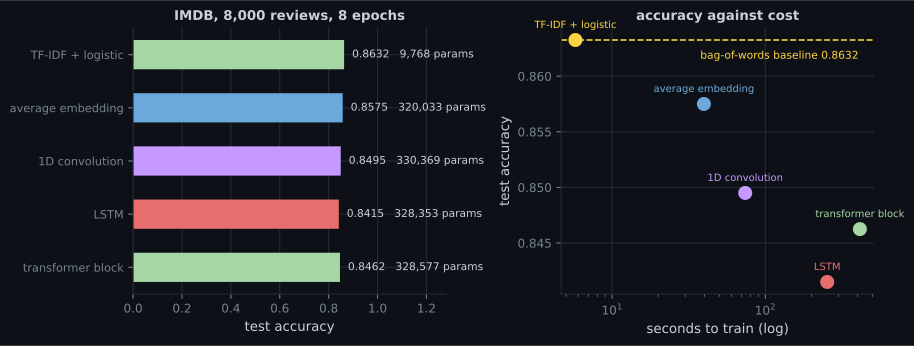
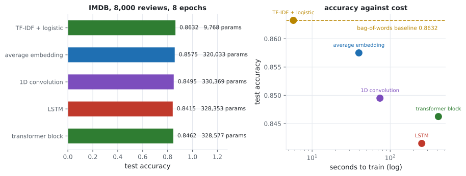
Three reasons the ordering comes out this way, and none of them is “neural networks don’t work”:

The task is decidable from word presence. “Terrible”, “waste”, “excellent” are near-deterministic signals in a movie review. Order helps at the margins — not good — but the margins are small.
8,000 reviews is not much data. A linear model over 10,000 sparse features has effectively one parameter per word and a strong inductive bias; a transformer has 328,577 parameters and no prior about text at all.
The sequence models see a truncated review. Every neural family here reads 200 tokens; the TF-IDF model reads the entire review. That is a real advantage and it is part of why the baseline is hard to beat.

The ranking depends on the data budget

Training rows	TF-IDF + logistic	Average embedding	LSTM
1,000	0.8190	0.7258	0.7530
4,000	0.8485	0.8255	0.8225
8,000	0.8632	0.8575	0.8415

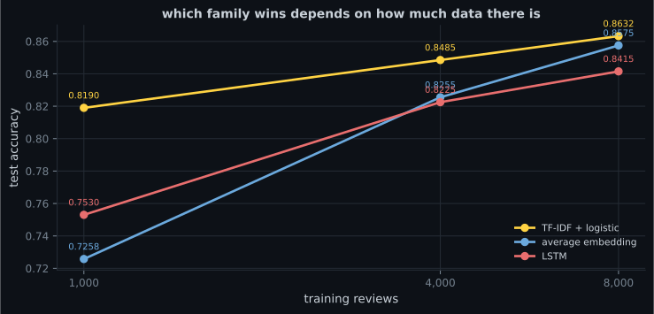
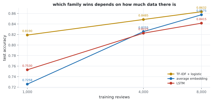
Three lines of test accuracy against training reviews on a log axis. TF-IDF plus logistic starts highest at 0.8190 with 1,000 rows and stays highest through 0.8632 at 8,000. The average embedding rises steeply from 0.7258 and nearly catches up. The LSTM rises from 0.7530 to 0.8415 and remains lowest at the largest size. — The gap is widest where data is scarcest: 0.0932 over the average embedding at 1,000 rows, closing to 0.0057 at 8,000. Extrapolate the slopes and the neural families overtake somewhere past this chart — which is exactly the regime the published results come from. The honest statement is not 'bag of words is better' but 'bag of words is better here, and the crossover is a data-budget question'.

The neural curves are steeper. That is the whole argument for them: they have more capacity to use once there is enough data to constrain it, and less useful prior when there is not.

Is the confidence meaningful?

An accuracy figure says how often the model is right. It says nothing about whether 0.9 means nine times out of ten. For the winning model:

Predicted band	Reviews	Observed positive rate
0.0 – 0.2	838	0.0095
0.2 – 0.4	774	0.1266
0.4 – 0.6	747	0.4632
0.6 – 0.8	947	0.8427
0.8 – 1.0	694	0.9784

Two panels. Left: bars over 4,000 test reviews — both models right 3,327, only the average embedding right 103, only the bag of words right 126, both wrong 444. Right: a reliability curve of observed positive rate against predicted probability, tracking the diagonal closely, with the count of reviews in each band annotated. — The two models differ by 0.0057 overall and disagree on 229 reviews — 103 that only the embedding model gets and 126 that only the bag of words gets. An oracle choosing the better model per review would score 0.8890 against the best single model's 0.8632, which is the entire case for ensembling and is invisible in a single accuracy number. The reliability curve is close to the diagonal: reviews scored 0.8-1.0 really are positive 97.84% of the time.

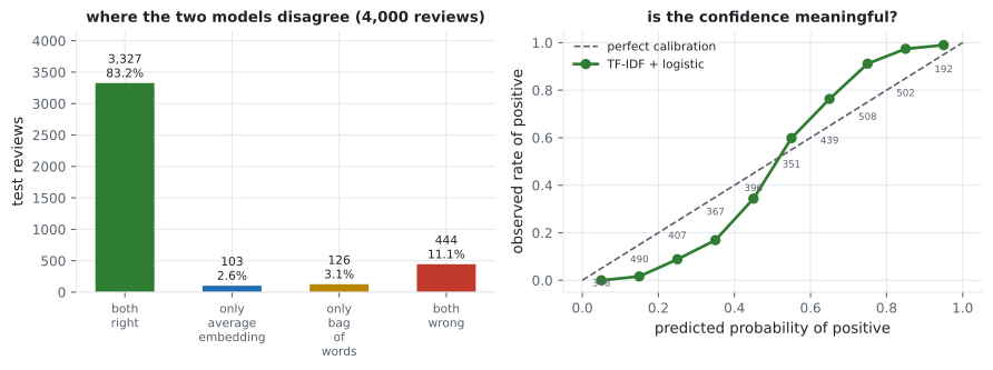
Logistic regression is calibrated almost by construction — it optimises log loss, which is a proper scoring rule. Neural classifiers trained with the same loss often are not, because they are flexible enough to become overconfident; that is what temperature scaling on a validation set is for.

What this page does not show

A tuned transformer. One block, 32 dimensions, 8 epochs, from scratch. Published transformer results on IMDB use pretrained models with 10⁸ parameters — a different experiment entirely.
Longer inputs. All neural families truncate to 200 tokens, which discards 43.86% of reviews’ content by the measurement on the preprocessing page.
A harder task. Sentiment is close to a keyword problem. Nothing here is evidence about tasks that genuinely need composition — negation scope, coreference, multi-hop reasoning.

diagram Diagram mermaid

  flowchart TB
  A["text classification task"] --> B["TF-IDF + logistic regression
8.4s, 0.8632"]
  B --> C{"good enough?"}
  C -->|"yes"| D["ship it — and keep it
as the baseline"]
  C -->|"no"| E{"why not?"}
  E -->|"needs word order"| F["sequence or attention model"]
  E -->|"needs more data"| G["the neural curves are steeper"]
  E -->|"needs world knowledge"| H["a pretrained model"]
  F --> I["measure against B again"]
  G --> I
  H --> I

sketch Accuracy against cost p5.js

The five families as measured. Drag the slider to weight accuracy against training time and see which family a given trade-off picks.

sketch The measured table, ranked p5.js

Click a column to rank every row by it. The bars are that column's values and the highest and lowest are computed from the numbers, not written in.

Pitfalls

Skipping the linear baseline. It won here, in 8.4 seconds. A neural result that was never compared against it is not a result.
Comparing families at different input lengths. The TF-IDF model read whole reviews; the neural ones read 200 tokens. Say so, or equalise it.
Reading one dataset size as the ranking. The gap over the average embedding was 0.0932 at 1,000 rows and 0.0057 at 8,000.
Quoting accuracy without calibration. Both matter, and they are different properties; a model can be accurate and badly calibrated.
Calling a one-block 32-dimensional encoder “a transformer”. Published results use pretrained models three orders of magnitude larger.
Tuning the neural model and not the baseline. Sublinear TF-IDF was worth +0.0216 on the previous page for one keyword.
Assuming the ordering transfers. Sentiment is nearly a keyword task; negation scope and coreference are not.

Recap

Five families, one split: TF-IDF + logistic 0.8632 in 8.4 s, average embedding 0.8575, 1D convolution 0.8495, transformer 0.8462, LSTM 0.8415.
The winner used 9,768 parameters against the transformer’s 328,577, and trained 55× faster.
The accuracy spread across all five families was 0.0217; the cost spread was 55×.
The advantage is largest at small data: +0.0932 over the average embedding at 1,000 rows, +0.0057 at 8,000.
The winner is well calibrated: predicted 0.8–1.0 corresponds to an observed 0.9784 positive rate.
Neural curves are steeper, so the crossover is a data-budget question — not a statement that sequence models do not work.
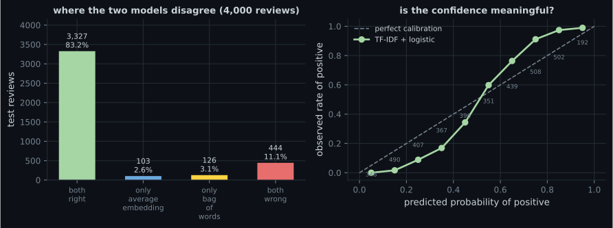
The two closest models disagree on 229 of 4,000 reviews; an oracle picking the better one per review would score 0.8890 against 0.8632.

Attention was measured on its own; the full architecture — blocks, residuals, normalisation, positions — is next, with an ablation for each part: The Transformer Architecture.

pch.quizTag pch.quizDefaultTitle

TF-IDF with logistic regression scored 0.8632 while a transformer block scored 0.8462 in 55x the time. What is the right conclusion?

pch.quizShowAnswer

B — On this task and this data budget the linear model wins — sentiment is close to a keyword problem, 8,000 reviews is little data, and the baseline reads whole reviews while the neural models truncate to 200 tokens — The neural curves are steeper with data, so the crossover is a budget question. Published transformer results on IMDB use pretrained models with 10^8 parameters.
At 1,000 training rows the gap over the average embedding was 0.0932; at 8,000 it was 0.0057. What does that trend suggest?

pch.quizShowAnswer

B — The neural family has more capacity and a weaker prior, so it improves faster with data — extrapolating, it overtakes past the largest size measured here — This is why a single dataset size is not a ranking, and why the honest claim is about the regime rather than the architecture.
The winning model's 0.8-1.0 confidence band contained reviews that were positive 97.84% of the time. What property is that?

pch.quizShowAnswer

B — Calibration — the predicted probabilities can be read as probabilities, which is what makes a threshold on top of them meaningful — Logistic regression optimises log loss, a proper scoring rule, so it tends to be calibrated. Flexible neural classifiers often are not, which is what temperature scaling fixes.
All the neural families truncated reviews to 200 tokens while the TF-IDF model read the whole review. Why does that matter?

pch.quizShowAnswer

B — It is an uncontrolled difference in the comparison — 43.86% of reviews are longer than 200 tokens, so the baseline had strictly more information — Either equalise it or state it. This page states it, because equalising would make the neural models much slower still.
What is the most useful thing to do with a linear baseline that beats your neural model?

pch.quizShowAnswer

B — Keep it as the reference every later model must beat, and use the disagreement between them to find what the neural model is actually adding — A model that only wins by 0.01 overall may still be right about a very different 1% — which is worth knowing before choosing one.

🧪 Try It Yourself

pch.coffeeTagline

pch.coffeeCta

pch.feedbackHeading

pch.feedbackSubheading