What you’ll learn

• the three paradigms separated by one question: what feedback does the learner receive?
• semi-supervised learning, and a case where 20 labels reach 1.0000 on 600 points
• batch vs online under drift, measured: mean accuracy 0.7391 against 0.9705
• instance-based vs model-based: 2 numbers stored, or all 26 rows
• which of the four axes actually determines your algorithm choice

The organising question

Textbooks list the paradigms as though they were arbitrary categories. They are not. There is one question underneath, and everything else follows from the answer.

What feedback does the learner get after it acts?

  flowchart TD
  Q["After the learner acts,
what does it find out?"]
  Q -->|"the right answer, always"| S["SUPERVISED
regression · classification"]
  Q -->|"nothing"| U["UNSUPERVISED
clustering · dimensionality reduction"]
  Q -->|"a reward, delayed"| R["REINFORCEMENT
policy learning"]
  Q -->|"the right answer, rarely"| SS["SEMI-SUPERVISED
label propagation"]

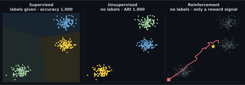
Here are the first three on the same 300 points, so the difference is visible rather than described:

figureSame points, three kinds of feedbackmatplotlib

1. Supervised learning

You have inputs $X$ and correct outputs $y$. The model learns the mapping.

Two sub-types, distinguished only by what $y$ looks like:

This is the overwhelming majority of deployed machine learning, and it is where the labelling cost lives. Somebody has to produce $y$ for every training row.

2. Unsupervised learning

You have $X$ and nothing else. The algorithm finds structure — groups, directions, densities — and there is no answer key to check it against.

That absence is the defining difficulty. On the figure above, unsupervised clustering scored an adjusted Rand index of 1.0000 against the hidden labels, but only because we had those labels to check with. In a real unsupervised problem you would never know.

3. Reinforcement learning

An agent takes actions in an environment, which returns a new state and a reward. The agent learns a policy — a mapping from states to actions — that maximises cumulative reward.

  flowchart LR
  A["Agent"] -->|"action a"| E["Environment"]
  E -->|"new state s'"| A
  E -->|"reward r"| A

Two things make this genuinely harder than supervised learning:

Credit assignment. You lose a chess game after 60 moves. Which move was the mistake? The reward arrives once, at the end, for a long sequence of decisions.

Exploration versus exploitation. The agent only learns about actions it tries. Always taking the best-known action means never discovering a better one.

Reinforcement learning is not covered further in this module — it needs an environment to interact with, not a dataset — but you should recognise it. Game-playing agents, robot control, and some recommendation and ad-bidding systems are RL.

4. Semi-supervised learning

Labels are expensive; unlabelled data is usually free. Semi-supervised methods use both: a few labels to anchor the classes, and the geometry of the unlabelled mass to fill in the rest.

Measured on 600 two-moons points with only 20 labelled:

figureTwenty labels are plenty — if the model can express the shapematplotlib

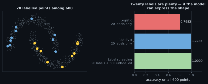
The honest reading of that table matters. Label spreading wins, but by 0.0067 over a supervised model with the right inductive bias. The dramatic gap is between logistic regression (0.7983) and everything else — and that gap is about model shape, not label count. Semi-supervised learning is genuinely useful, and it is not the biggest lever in this table.

Cross-cutting axis 1: batch or online

Independent of the paradigm: does the model learn once, or continuously?

Batch (offline) learning trains on all available data, deploys, and stops learning. To incorporate new data you retrain from scratch.

Online (incremental) learning updates from each new batch as it arrives, via partial_fitpartial_fit.

  flowchart TD
  subgraph B["Batch learning"]
    B1["Train on everything"] --> B2["Deploy — frozen"]
    B2 -.->|"new data"| B3["Retrain from scratch"] --> B2
  end
  subgraph O["Online learning"]
    O1["partial_fit on a chunk"] --> O2["Deploy, keep learning"]
    O2 -->|"new data"| O1
  end

The distinction is invisible on static data and decisive when the world moves. Here is a stream where the true decision boundary rotates 3.2° per chunk — a slow, unremarkable drift — with each model scored on the next chunk before it sees it:

figureWhen the world drifts, only one of these keeps upmatplotlib

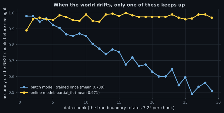
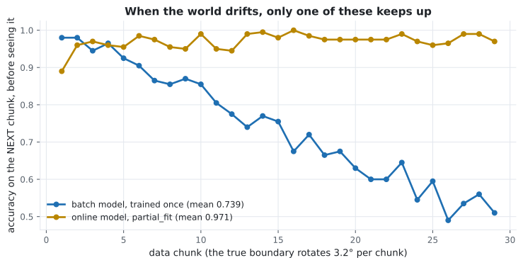
The batch model does not break. It stays exactly as correct as it was on the day it was trained, while the world stops matching it. Nothing alerts. This is the single most important reason monitoring exists.

Online learning is not free: it can be corrupted by bad incoming data, it is harder to reproduce, and rolling it back means restoring a snapshot of the weights. A scheduled batch retrain is often the right compromise.

Cross-cutting axis 2: instance-based or model-based

Also independent of the paradigm: does the algorithm generalise or memorise?

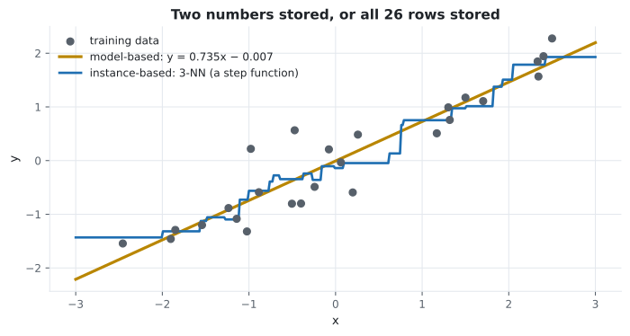
Model-based learners compress the training data into parameters and then discard the data. A linear model on 26 points stored 2 numbers: coefficient 0.7348, intercept −0.0070.

Instance-based learners keep the examples and compare new inputs against them at prediction time. 3-NN on the same 26 points stored all 26 rows and learned no parameters at all.

figureTwo numbers stored, or all 26 rows storedmatplotlib

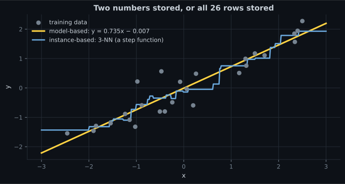
Watch the two readouts at the top. The model-based number slides smoothly, because it is a straight line evaluated at a moving point. The instance-based number jumps whenever the set of three nearest neighbours changes — it is an average over whichever rows happen to be closest.

Putting the axes together

Four independent choices, and only one of them is usually forced by the problem:

The first two are dictated. Spend your judgement on the last two.

In code

All three paradigms, side by side:

from sklearn.cluster import KMeans
from sklearn.datasets import make_blobs
from sklearn.linear_model import LogisticRegression
from sklearn.metrics import adjusted_rand_score
 
X, y = make_blobs(n_samples=300, centers=3, cluster_std=1.1, random_state=8)
 
# Supervised: y is available, so learn the mapping X -> y.
supervised = LogisticRegression(max_iter=1000).fit(X, y)
print("supervised accuracy", round(supervised.score(X, y), 4))       # 1.0
 
# Unsupervised: pretend y does not exist. Find structure in X alone.
labels = KMeans(n_clusters=3, n_init=10, random_state=0).fit_predict(X)
print("unsupervised ARI   ", round(adjusted_rand_score(y, labels), 4))  # 1.0
# ^ we can only compute that ARI because we secretly kept y.
#   In a real unsupervised problem there is nothing to compare against.

from sklearn.cluster import KMeans
from sklearn.datasets import make_blobs
from sklearn.linear_model import LogisticRegression
from sklearn.metrics import adjusted_rand_score
 
X, y = make_blobs(n_samples=300, centers=3, cluster_std=1.1, random_state=8)
 
# Supervised: y is available, so learn the mapping X -> y.
supervised = LogisticRegression(max_iter=1000).fit(X, y)
print("supervised accuracy", round(supervised.score(X, y), 4))       # 1.0
 
# Unsupervised: pretend y does not exist. Find structure in X alone.
labels = KMeans(n_clusters=3, n_init=10, random_state=0).fit_predict(X)
print("unsupervised ARI   ", round(adjusted_rand_score(y, labels), 4))  # 1.0
# ^ we can only compute that ARI because we secretly kept y.
#   In a real unsupervised problem there is nothing to compare against.

Online learning, and what it costs to skip it:

import numpy as np
from sklearn.linear_model import LogisticRegression, SGDClassifier
 
rng = np.random.default_rng(0)
 
def chunk(i, per=200):
    """The true boundary rotates 3.2 degrees with every chunk."""
    angle = np.radians(3.2 * i)
    X = rng.normal(0, 1, (per, 2))
    w = np.array([np.cos(angle), np.sin(angle)])
    return X, (X @ w > 0).astype(int)
 
X0, y0 = chunk(0)
batch = LogisticRegression().fit(X0, y0)          # trained once, never again
online = SGDClassifier(loss="log_loss", random_state=0)
online.partial_fit(X0, y0, classes=np.array([0, 1]))
 
batch_scores, online_scores = [], []
for i in range(1, 30):
    Xi, yi = chunk(i)
    batch_scores.append(batch.score(Xi, yi))
    online_scores.append(online.score(Xi, yi))    # score BEFORE updating
    online.partial_fit(Xi, yi)                    # then learn from it
 
print(f"batch  mean {np.mean(batch_scores):.4f}  last {batch_scores[-1]:.4f}")
print(f"online mean {np.mean(online_scores):.4f}  last {online_scores[-1]:.4f}")
# batch  mean 0.7391  last 0.5100
# online mean 0.9705  last 0.9700

import numpy as np
from sklearn.linear_model import LogisticRegression, SGDClassifier
 
rng = np.random.default_rng(0)
 
def chunk(i, per=200):
    """The true boundary rotates 3.2 degrees with every chunk."""
    angle = np.radians(3.2 * i)
    X = rng.normal(0, 1, (per, 2))
    w = np.array([np.cos(angle), np.sin(angle)])
    return X, (X @ w > 0).astype(int)
 
X0, y0 = chunk(0)
batch = LogisticRegression().fit(X0, y0)          # trained once, never again
online = SGDClassifier(loss="log_loss", random_state=0)
online.partial_fit(X0, y0, classes=np.array([0, 1]))
 
batch_scores, online_scores = [], []
for i in range(1, 30):
    Xi, yi = chunk(i)
    batch_scores.append(batch.score(Xi, yi))
    online_scores.append(online.score(Xi, yi))    # score BEFORE updating
    online.partial_fit(Xi, yi)                    # then learn from it
 
print(f"batch  mean {np.mean(batch_scores):.4f}  last {batch_scores[-1]:.4f}")
print(f"online mean {np.mean(online_scores):.4f}  last {online_scores[-1]:.4f}")
# batch  mean 0.7391  last 0.5100
# online mean 0.9705  last 0.9700

Note partial_fitpartial_fit needs classes=classes= on its first call — it cannot infer the full label set from one chunk.

Pitfalls

Calling a problem unsupervised because the labels are inconvenient to collect. If you can get labels, get them. Supervised learning is enormously easier to evaluate.

Evaluating unsupervised results against labels you secretly have and pretending that generalises. The ARI of 1.0000 above required the hidden yy. Real unsupervised work has no such check — see the clustering page.

Assuming a batch model stays correct. Measured: 0.9800 down to 0.5100 with no error and no alert, from a drift of 3.2° per chunk.

Reaching for online learning by default. It is harder to reproduce, harder to roll back, and vulnerable to poisoned inputs. Scheduled retraining solves most drift.

Forgetting instance-based models carry the data. A k-NN model is a data export. That has storage, latency and sometimes privacy consequences.

Believing semi-supervised learning is always the answer to few labels. Measured above: an RBF SVM on 20 labels alone got 0.9933 against label spreading’s 1.0000. Try the supervised model with the right inductive bias first.

Recap

• One question separates the paradigms: what feedback does the learner get?
• Supervised needs labels; unsupervised has no answer key at all; RL gets a delayed reward.
• Semi-supervised reached 1.0000 from 20 labels, but a well-chosen supervised model got 0.9933 from the same 20 — the real gap was model shape, not label count.
• Under 3.2°-per-chunk drift, a batch model fell from 0.9800 to 0.5100 (mean 0.7391) while an online model held at 0.9705.
• Model-based stores parameters (2 numbers); instance-based stores the data (26 rows).
• The first two axes are dictated by your data. The last two are your judgement.

🧪 Try It Yourself

Exercise 1 – The same data, with and without labels

Exercise 2 – Watch a batch model rot

Exercise 3 – Online learning keeps up

Exercise 4 – Two numbers, or all the rows

Exercise 5 – Twenty labels, three approaches

Exercise 6 – One line separates a batch model from an online one

Next

The ML Lifecycle - From Data to Deployment — the eight stages of a real project, and the measurement showing that changing the algorithm and damaging the labels move accuracy by exactly the same amount.