The Universal Workflow of Machine Learning

Every technique in this phase was measured in isolation. A real project needs an order to apply them in, and that order matters more than the techniques do: most failed projects fail at step 1, on a task that was never framed properly or a baseline that was never measured. This page runs the whole workflow on one dataset and reports what each step bought.

What you’ll learn

• A five-rung baseline ladder measured end to end: 0.1015 → 0.8400 → 0.8580 → 0.8595 → 0.8635.
• Why the 26× parameter jump from rung 3 to rung 4 bought 0.0015.
• The overfit-then-regularise step with numbers: gaps of 0.0221, 0.0981 and 0.0516 for three capacities.
• The one-batch smoke test: 32 rows memorised to accuracy 1.0000 with 256 units, 0.8750 with 4.
• The sanity checks worth running before any model exists.
• Which last layer and loss to pair with each kind of target.

Step 1: define the task

Before code: what is predicted, from what, and what does being wrong cost?

diagram Diagram mermaid

  flowchart TD
  A["1. define the task"] --> B["what are the inputs?
what is the target?
what does a mistake cost?"]
  B --> C["pick a metric
and a loss that has a gradient"]
  C --> D["2. develop a model"]
  D --> E["beat a dumb baseline"]
  E --> F["build something that overfits"]
  F --> G["regularise and tune"]
  G --> H["3. deploy"]
  H --> I["monitor drift, retrain,
keep the test set untouched"]

The choice of last layer and loss is mechanical once the target is described:

Target	Last layer	Loss	Metric to report
binary	Dense(1, "sigmoid")	binary_crossentropy	accuracy, or precision/recall
multiclass, one label	Dense(K) + from_logits=True	sparse_categorical_crossentropy	accuracy and macro recall
multiclass, many labels	Dense(K, "sigmoid")	binary_crossentropy	per-label F1
continuous	Dense(1)	mse or huber	MAE, in the target’s units
bounded continuous [0,1]	Dense(1, "sigmoid")	mse or binary_crossentropy	MAE

The reasoning behind each pairing — and the from_logits trap — is on the loss functions page.

Sanity checks before any model exists

Five minutes that save a day

print(x.shape, x.dtype, x.min(), x.max(), x.mean())
print(np.isnan(x).sum(), np.isinf(x).sum())
print(np.bincount(y))                                    # class balance
print(len(x) - len(np.unique(x, axis=0)))                # duplicate rows

Measured on 8,000 Fashion-MNIST rows: range [0.0000, 1.0000], mean 0.2851, zero NaNs, class counts from 747 to 860 — near-balanced, so the majority baseline is 0.1075 — and 0 duplicate rows. Every one of those four numbers changes what you do next. A class count of 7,900 against 100 changes the metric; duplicate rows change the split, as the evaluation page measured at 0.9600 accuracy on pure noise.

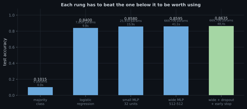
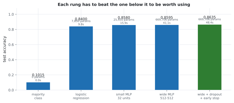
Step 2a: beat a dumb baseline

Each rung has to justify itself against the one below. Fashion-MNIST, 8,000 training rows, one held-out test set, everything measured:

figure Each rung has to beat the one below it to be worth using matplotlib

The first two rungs cover 0.7385 of the total climb; everything after them adds 0.0235 between them. The 512-512 model has 26 times the parameters of the 32-unit model and beat it by 0.0015 — inside noise. Only after adding dropout and early stopping does the wide model earn its size, at 0.8635.

Rung	Test accuracy	Parameters	Seconds
majority class	0.1015	0	0.00
logistic regression	0.8400	7,850	21.57
MLP, 32 units	0.8580	25,450	15.27
MLP, 512-512	0.8595	669,706	42.26
512-512 + dropout 0.4 + early stopping	0.8635	669,706	34.56

Read the ladder as a cost-benefit table, not a leaderboard:

• Rung 2 does most of the work. Logistic regression covers 0.7385 of the 0.7620 total climb, with 7,850 parameters and no tuning.
• Rung 4 is not worth its price on its own. 26× the parameters of rung 3 for 0.0015 accuracy — smaller than the noise on this test set.
• Rung 5 is where the extra capacity pays, and only because it is regularised: 0.8635, and it trained faster than rung 4 because early stopping cut it short.
• The whole neural network contribution is 0.0235 over logistic regression. That is real and it is small, and knowing the size of it is the point of building the ladder.

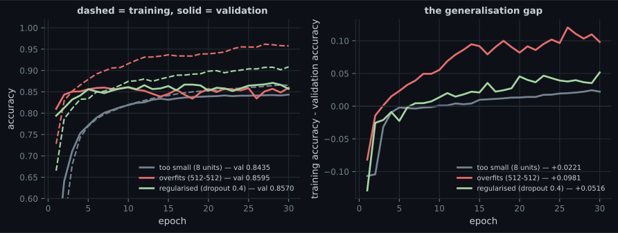
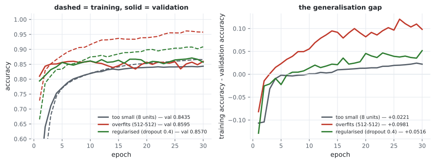
Step 2b: build something that overfits, then push back

The recommended order is deliberately counter-intuitive: first make the model bad in the right direction. A model that cannot overfit has no headroom to regularise, and you cannot tell an underfitting model from a badly tuned one.

figure Three capacities, one dataset matplotlib

The 8-unit model has a gap of 0.0221 and cannot do better — it is underfitting, and no regulariser helps. The 512-512 model reaches a gap of 0.0981, which is the signal that there is headroom to trade. Adding dropout 0.4 cuts the gap to 0.0516 and produces the best validation accuracy of the three at its best epoch: 0.8710.

Model	Train accuracy	Val accuracy	Gap	Best val accuracy
8 units (too small)	0.8656	0.8435	0.0221	0.8435
512-512 (overfits)	0.9576	0.8595	0.0981	0.8605
512-512 + dropout 0.4	0.9086	0.8570	0.0516	0.8710

The 8-unit row is the important one. Its gap is small, which looks healthy and is not: both numbers are low, and no amount of dropout, weight decay or scheduling will raise them. A small gap is only good news when the scores are high.

Note also that the regularised model’s final validation accuracy (0.8570) is slightly below the unregularised one’s (0.8595), while its best is clearly higher (0.8710 against 0.8605). With dropout the run is noisier epoch to epoch, so the best-epoch weights are what you want — which is exactly what EarlyStopping(restore_best_weights=True) gives you.

The one-batch smoke test

Before worrying about data, architecture or hyperparameters, check that the model can memorise a single batch. Take 32 rows, train for 200 epochs, and demand near-zero loss:

Hidden units	Final training loss on 32 rows	Accuracy
4	0.402435	0.8750
256	0.000253	1.0000

The 256-unit model memorises 32 rows perfectly, as it must — 200,000 parameters against 32 examples. If your model cannot do this, the problem is a bug: a mislabelled target, a broken preprocessing step, a frozen layer, a learning rate of zero. Data volume, regularisation and architecture are all irrelevant until this test passes.

The 4-unit model’s failure is informative in the other direction: it is not a bug, it is a capacity limit, and it stalls at 0.8750 on 32 rows.

The whole test

model.fit(x_train[:32], y_train[:32], epochs=200, batch_size=32)
# demand a loss near zero. If you cannot get it, stop and find the bug.

What “scale up until you overfit” looks like

The instruction is precise but the number is not obvious, so here is the sweep: six model sizes spanning 146×, no regularisation, everything else held fixed.

figure Fashion-MNIST, 8,000 rows, 30 epochs, no regularisation matplotlib

Read the two panels together. Training accuracy rises monotonically — the model is absorbing more of the training set at every size, exactly as intended. Validation accuracy does not: it moves 0.0150 in total across a 146x range of parameters, and not monotonically. The gap panel is the signal the instruction is pointing at: it nearly triples between 12,730 and 203,530 parameters, which is where this model starts memorising rather than learning.

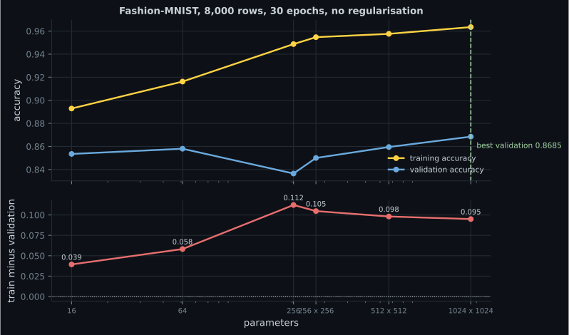
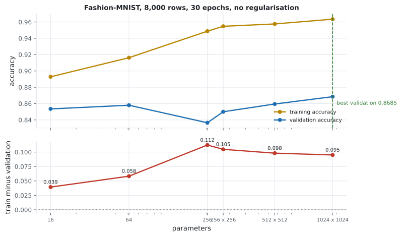
Model	Parameters	Train	Validation	Best validation	Gap
16	12,730	0.8929	0.8535	0.8540	0.0394
64	50,890	0.9162	0.8580	0.8600	0.0583
256	203,530	0.9488	0.8365	0.8540	0.1123
256 × 256	269,322	0.9548	0.8500	0.8685	0.1047
512 × 512	669,706	0.9576	0.8595	0.8605	0.0981
1024 × 1024	1,863,690	0.9635	0.8685	0.8725	0.0950

Two things worth taking from this that the instruction alone does not tell you.

Overfitting is not the same as getting worse. The largest model has both the biggest training–validation gap and the best validation accuracy. “Overfitting” describes the gap, not the outcome; a model can memorise heavily and still generalise best of the ones you tried.

146× the parameters bought 0.0150 of validation accuracy. If the search had stopped at 64 units it would have given up almost nothing and trained in a fraction of the time. The value of this sweep is knowing that — which you only know by running it.

Step 3: deploy, then keep measuring

One evaluation, once, at the end

loss, accuracy = model.evaluate(x_test, y_test)   # the first and only time

Three things belong in this step, and only the first is about modelling:

• Evaluate the test set exactly once. Every earlier number was used to make a decision and is therefore optimistic — measured on the IMDB page as 0.8882 validation against 0.8792 test.
• Save the whole model, not the weights. model.save("name.keras") carries the architecture, the weights and the non-trainable state that BatchNormalization layers depend on. A round trip reproduces predictions to 0.00e+00.
• Expect the input distribution to move. The model is a fixed function; the world is not. Log the input statistics you checked in step 1 and compare them periodically against the training set. A shifted mean is your early warning.

sketch Walk the ladder p5.js Pause Restart

The five measured rungs. Click one to see its accuracy against the rung below it, its parameter count, and whether the gain justified the cost.

sketch The measured table, ranked p5.js Pause Restart

Click a column to rank every row by it. The bars are that column's values and the highest and lowest are computed from the numbers, not written in.

Pitfalls

• Skipping the dumb baseline. Logistic regression covered 0.7385 of the total climb here. Without it, 0.8635 has no meaning.
• Starting from a big model. Rung 4’s 669,706 parameters beat rung 3’s 25,450 by 0.0015. Start small, grow only when the small model is clearly the limit.
• Regularising before overfitting. With a 0.0221 gap there is nothing to trade; the 8-unit model needed capacity, not dropout.
• Reading a small gap as healthy. It is only healthy when both scores are high.
• Skipping the one-batch smoke test. A model that cannot memorise 32 rows has a bug, and no amount of data or tuning will fix it.
• Choosing a metric that has no gradient. Train on a differentiable surrogate, report the metric you care about, and keep the two distinct.
• Touching the test set more than once. Every look costs you the guarantee it exists to provide.
• Assuming the deployed distribution is the training distribution. Log the step-1 statistics and re-check them on live data.

Recap

• Step 1 is framing: inputs, target, cost of error, then a mechanical choice of last layer and loss. Four cheap sanity checks come before any model.
• The measured ladder ran 0.1015 → 0.8400 → 0.8580 → 0.8595 → 0.8635, with logistic regression alone covering 0.7385 of the climb.
• Going from 25,450 to 669,706 parameters bought 0.0015 unregularised, and 0.0055 once dropout and early stopping were added.
• Overfit first: the 8-unit model’s 0.0221 gap was underfitting, the 512-512 model’s 0.0981 gap was the headroom, and dropout converted it into a best-epoch 0.8710.
• The one-batch smoke test: 256 units memorised 32 rows to loss 0.000253 and accuracy 1.0000; 4 units stalled at 0.8750. Failing it means a bug.
• Deployment is one test-set evaluation, a full model.save, and ongoing comparison of live input statistics against the training set.

Next

The measurement discipline this page describes is what the rest of the phase supplies the tools for: Evaluating Models: Generalization and Validation covers how to make each rung’s number trustworthy in the first place.

pch.quizTag pch.quizDefaultTitle

1. Logistic regression scored 0.8400 and the final tuned network 0.8635 on the same data. Why build the logistic model at all?

   A As a fallback in case the network fails to train B Because it establishes the size of the network's contribution — 0.0235 — which is the only way to judge whether the extra parameters, training time and complexity are worth carrying C Because linear models generalise better D It is only needed when the dataset is small
   pch.quizShowAnswer

   B — Because it establishes the size of the network's contribution — 0.0235 — which is the only way to judge whether the extra parameters, training time and complexity are worth carrying — 0.8635 sounds impressive alone. Against 0.8400 from 7,850 untuned parameters, it is a modest and quantified gain.

2. A model reaches 0.8656 training accuracy and 0.8435 validation accuracy — a gap of only 0.0221. What should you do?

   A Nothing: a small gap means the model generalises well B Add capacity — both numbers are low, so the model is underfitting and there is nothing for a regulariser to trade against C Add dropout to close the gap further D Collect more training data
   pch.quizShowAnswer

   B — Add capacity — both numbers are low, so the model is underfitting and there is nothing for a regulariser to trade against — A small gap is only good news when the scores are high. This is why the workflow says overfit first, then push back.

3. Your model cannot get below 1.8 training loss on a single batch of 32 rows after 200 epochs. What is the most likely cause?

   A The dataset is too small overall B A bug — mislabelled targets, broken preprocessing, a frozen layer or a zero learning rate — because a model with enough parameters must be able to memorise 32 examples C The model needs more regularisation D The batch size is too small
   pch.quizShowAnswer

   B — A bug — mislabelled targets, broken preprocessing, a frozen layer or a zero learning rate — because a model with enough parameters must be able to memorise 32 examples — Measured: 256 units reached loss 0.000253 and accuracy 1.0000 on 32 rows. Failing that test is a bug, not a data or tuning problem.

4. Rung 4 (669,706 parameters) beat rung 3 (25,450 parameters) by 0.0015 accuracy. What is the right response?

   A Ship rung 4 — it has the higher score B Treat the difference as noise on a 2,000-row test set and keep the smaller model, unless regularisation turns the extra capacity into a real gain, as it did at rung 5 C Increase the model size further D Rerun rung 3 with a different seed until it wins
   pch.quizShowAnswer

   B — Treat the difference as noise on a 2,000-row test set and keep the smaller model, unless regularisation turns the extra capacity into a real gain, as it did at rung 5 — Rung 5 is the same architecture as rung 4 with dropout and early stopping, and it reached 0.8635 — the capacity only paid once it was constrained.

5. Why is the last-layer-and-loss choice described as mechanical rather than a design decision?

   A Because Keras picks it automatically B Because it follows from the target's type: a bounded probability needs sigmoid and cross-entropy, one-of-K needs softmax, an unbounded number needs a linear output — the pairings exist so the gradient behaves C Because any loss works if you train long enough D Because the metric and the loss are always the same function
   pch.quizShowAnswer

   B — Because it follows from the target's type: a bounded probability needs sigmoid and cross-entropy, one-of-K needs softmax, an unbounded number needs a linear output — the pairings exist so the gradient behaves — The sigmoid-plus-cross-entropy gradient reduces to (prediction - target). Mismatching the pairing removes that cancellation and the model stops learning from confident errors.

🧪 Try It Yourself

pch.exerciseTag pch.exerciseTitle

pch.exerciseTag pch.exerciseTitle

pch.exerciseTag pch.exerciseTitle

pch.exerciseTag pch.exerciseTitle

pch.exerciseTag pch.exerciseTitle

pch.exerciseTag pch.exerciseTitle