Building Neural Networks with Keras (Sequential and Functional API)

Keras offers three ways to define a model. Choosing between them is not a performance decision — the same architecture through all three produces bit-identical predictions and trains in the same time to within 2%. It is a decision about what the framework can see, and therefore what it can do for you.

What you’ll learn

• Sequential, Functional and Subclassing side by side: 5,121 parameters each, predictions matching to 0.00e+00, training times within 0.12s of each other.
• What subclassing gives up: count_params() raises on a fresh model, then reports 0 even after build() — only a forward pass sizes the kernels.
• A Functional-only architecture (wide & deep) measured: 13 extra parameters for 0.0431 better test MAE.
• compile / fit / evaluate / predict — the four verbs, identical across all three APIs.
• Four stopping policies on the same model: 2.8941 down to 2.7653 test MAE, and why restore_best_weights=True is the line that matters.
• Saving: a .keras file reproduces predictions to 0.00e+00 and carries the optimizer state with it.

The same model, three spellings

A two-hidden-layer regressor for the house-price data, written three ways.

Sequential: a list of layers

from tensorflow import keras
 
def sequential_model():
    return keras.Sequential([
        keras.layers.Input((13,)),
        keras.layers.Dense(64, activation="relu", name="h1"),
        keras.layers.Dense(64, activation="relu", name="h2"),
        keras.layers.Dense(1, name="out"),
    ])

Functional: call layers on tensors

def functional_model():
    inputs = keras.Input((13,))
    h = keras.layers.Dense(64, activation="relu", name="h1")(inputs)
    h = keras.layers.Dense(64, activation="relu", name="h2")(h)
    outputs = keras.layers.Dense(1, name="out")(h)
    return keras.Model(inputs, outputs)

Subclassing: write the forward pass yourself

class Subclassed(keras.Model):
    def __init__(self):
        super().__init__()
        self.h1 = keras.layers.Dense(64, activation="relu")
        self.h2 = keras.layers.Dense(64, activation="relu")
        self.out = keras.layers.Dense(1)
 
    def call(self, inputs):
        return self.out(self.h2(self.h1(inputs)))

With the same seed, all three are the same model:

	Parameters	Weight tensors	Max prediction difference vs Sequential
Sequential	5,121	6	—
Functional	5,121	6	0.00e+00
Subclassing	5,121	6	0.00e+00

The parameter count checks out by hand: $13 \times 64 + 64 = 896$, then $64 \times 64 + 64 = 4{,}160$, then $64 \times 1 + 1 = 65$, totalling 5,121. Six weight tensors is three kernels and three bias vectors.

Training time, 40 epochs at batch 16 on 404 rows:

API	Seconds	Test MAE
Sequential	5.55	2.8923
Functional	5.43	2.8923
Subclassing	5.52	2.8923

Identical accuracy, a 2% spread in time that is measurement noise. The API choice costs nothing and buys nothing at runtime. What differs is what happens before you call fit.

What each API actually gives you

diagram Diagram mermaid

  flowchart TD
  A["what does your model look like?"] --> B{"one input, one output,
layers in a line?"}
  B -- yes --> C["Sequential
shortest to write"]
  B -- no --> D{"can you draw it
as a static graph?"}
  D -- yes --> E["Functional
branches, merges, multiple I/O,
plot_model works"]
  D -- "no: loops, conditionals,
shape-dependent logic" --> F["Subclassing
arbitrary Python in call()"]

Sequential and Functional build a static graph that Keras can inspect. That is why model.summary() prints shapes, keras.utils.plot_model draws a diagram, and layer reuse is checkable. The Functional model exposes its graph directly:

python

print([layer.name for layer in functional_model().layers])
# ['input_layer_1', 'h1', 'h2', 'out']
print(sequential_model().input_shape)   # (None, 13)

Subclassing gives up that visibility, because call() is arbitrary Python and Keras cannot know what it does without running it. Measured on Keras 3.15:

python

model = Subclassed()
model.count_params()
# ValueError: You tried to call `count_params` on layer '<name>',
# but the layer isn't built.
 
model.build((None, 13))
print(model.count_params())     # 0
model.summary()                 # every layer shows "?" and "0 (unbuilt)"
 
model(np.zeros((1, 13), dtype="float32"))
print(model.count_params())     # 5,121

Three distinct states, and the middle one is the surprise. A fresh subclassed model raises rather than reporting zero. Model.build then marks the model itself built without propagating the shape into the sublayers, so count_params() answers 0 — technically accurate and thoroughly misleading. Only an actual forward pass sizes the kernels and gives 5,121.

The reason is that Dense(64) cannot allocate a $13 \times 64$ kernel until it knows the input has 13 columns, and the only thing that reveals that in a subclassed model is data flowing through call(). Sequential and Functional learn it from Input((13,)) at construction time, which is why they report 5,121 immediately.

The trade is real but narrow: use Sequential by default, Functional when the graph branches, and Subclassing only when the forward pass genuinely needs control flow that a graph cannot express.

What Functional buys: wide & deep

Some architectures cannot be written as a list. A wide & deep model sends the raw input both through the hidden layers and straight to the output:

A branch and a merge — impossible in Sequential

def wide_and_deep():
    inputs = keras.Input((13,))
    deep = keras.layers.Dense(64, activation="relu")(inputs)
    deep = keras.layers.Dense(64, activation="relu")(deep)
    joined = keras.layers.Concatenate()([inputs, deep])
    outputs = keras.layers.Dense(1)(joined)
    return keras.Model(inputs, outputs)

Measured against the plain stack, both trained 80 epochs at batch 16 on all 404 rows:

Model	Parameters	Test MSE	Test MAE
plain 64-64	5,121	17.8460	2.6112
wide & deep	5,134	16.7008	2.5681

13 extra parameters — one weight per raw feature reaching the output layer — for 0.0431 better MAE and 1.15 better MSE. That is a small, real gain from an architecture Sequential cannot express: the output layer sees both the learned representation and the untransformed features, so simple linear relationships do not have to survive two ReLU layers to reach it.

Treat the size of that gain honestly. It is roughly 1.7% of the MAE, on 102 test houses, from one run. The reason to know the pattern is that the same skip idea scales into residual networks in Phase 3, where it is the difference between trainable and untrainable.

sketch Build a Functional graph, watch the parameter count p5.js Pause Restart

Toggle the wide path and change the deep widths. The parameter count is computed exactly as Keras would: inputs times units plus units, per layer.

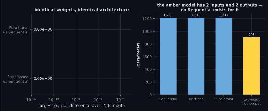
The three APIs produce the same model

“Sequential, Functional and subclassing are three ways to say the same thing” is easy to assert and easy to check: build one architecture three ways, copy identical weights into all three, and compare their outputs on the same 256 inputs.

figure Same architecture, same weights, 256 inputs matplotlib

Both differences are exactly 0.00e+00 — not 'small', zero — and all three report 1,217 parameters. The choice of API is a choice of notation. The amber bar is the exception that matters: a model with 2 inputs and 2 outputs, which Sequential cannot express at all because a Sequential model is by definition one chain from one input to one output.

Comparison	Largest output difference	Parameters
Functional vs Sequential	0.00e+00	1,217 vs 1,217
Subclassed vs Sequential	0.00e+00	1,217 vs 1,217
Two-input, two-output model	—	908

Pick the API by what you need to express, not by what you expect it to compute. Sequential until you need a branch; Functional when you do; subclassing when the forward pass has control flow that a graph of layers cannot describe.

Four verbs, identical everywhere

Whichever API built the model, the training interface is the same:

compile, fit, evaluate, predict

model.compile(optimizer="rmsprop", loss="mse", metrics=["mae"])
history = model.fit(x_train, y_train, epochs=80, batch_size=16,
                    validation_data=(x_val, y_val), verbose=0)
mse, mae = model.evaluate(x_test, y_test, verbose=0)
predictions = model.predict(x_test, verbose=0)

• compile attaches the optimizer, loss and metrics. It creates no weights and runs no data through the model.
• fit trains and returns a History whose .history is a plain dict of lists, one entry per metric per epoch.
• evaluate returns the loss followed by every metric, in compile order.
• predict returns raw model output — probabilities for a sigmoid or softmax head, unbounded numbers for a linear one.

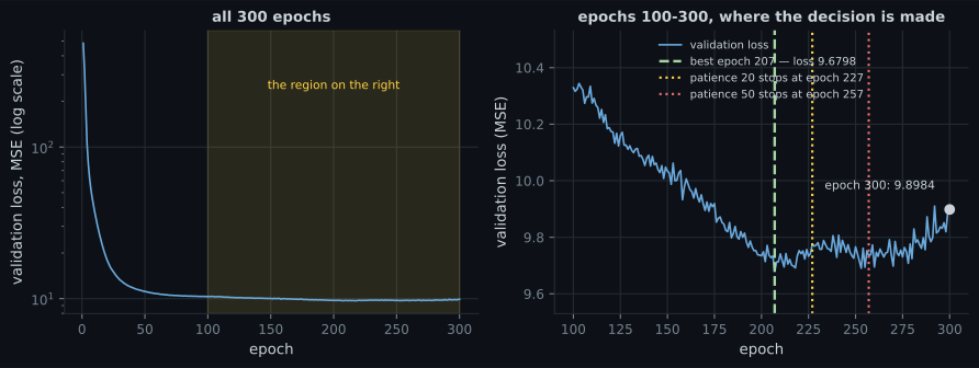
Callbacks: where the real decisions live

Fixed-epoch training forces you to guess. EarlyStopping watches a metric and stops when it stops improving. It has two parameters that matter, and one of them is routinely left at the wrong default.

figure 300 epochs of validation loss, and where patience fires matplotlib

Everything after epoch 100 happens in a band 0.8 MSE wide, which is why the left panel needs a log axis and the right panel needs a crop. The minimum, 9.6798, arrives at epoch 207; by epoch 300 the loss is 9.8984. Patience 20 stops at epoch 227 and patience 50 at 257 — both after the minimum, which is the point of patience.

Stop when it stops improving — and go back

stop = keras.callbacks.EarlyStopping(monitor="val_loss", patience=20,
                                     restore_best_weights=True)
model.fit(x_train, y_train, epochs=300, batch_size=16,
          validation_data=(x_val, y_val), callbacks=[stop], verbose=0)

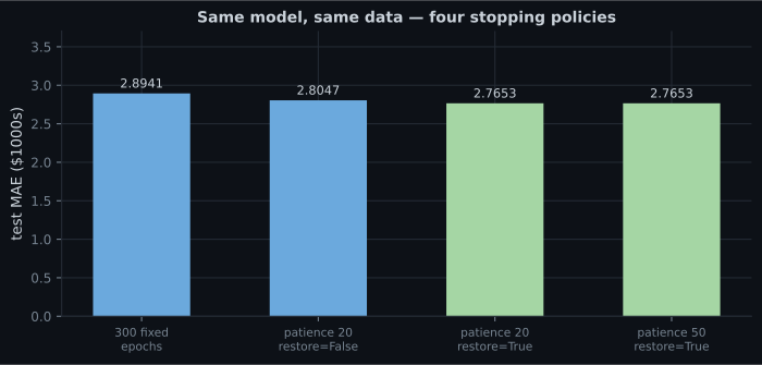
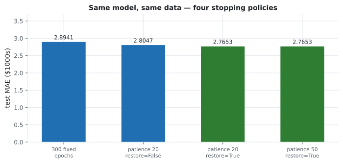
Four policies, the same model, the same seed, the same 320/84 split:

figure Same model, same data — four stopping policies matplotlib

Both restoring policies land on exactly 2.7653 because both roll back to the same epoch-207 weights; patience 50 simply spent 30 more epochs discovering nothing better. Stopping early without restoring gives back most of the benefit: 2.8047 against 2.7653.

Policy	Stopped after	Test MAE
300 fixed epochs	300	2.8941
patience 20, restore_best_weights=False	227	2.8047
patience 20, restore_best_weights=True	227	2.7653
patience 50, restore_best_weights=True	257	2.7653

Three readings:

1. restore_best_weights is the setting that matters, and it defaults to False. Without it, fit leaves you the weights from the last epoch — which is patience epochs past the best one, by construction. Here that costs 0.0394 MAE, and the whole point of the callback was to avoid exactly that.
2. Patience buys nothing extra once it is long enough. 20 and 50 both restore epoch 207 and score identically; patience 50 just burned 30 epochs.
3. Early stopping beat 300 fixed epochs by 0.1288 MAE. Modest, and the curve explains why: the plateau is nearly flat, so overtraining costs little here. On the IMDB model, where validation loss doubled after its minimum, the same callback is worth far more.

The honest caveat: that plateau is noisy. Between epochs 190 and 230 the validation loss wobbles by about 0.05 MSE, and “epoch 207” is partly which noise sample happened to be lowest. On a small validation set, the best epoch is an estimate, not a fact.

sketch Choose the patience, see where it fires p5.js Pause Restart

The real 300-epoch validation loss curve from the run above. Drag the slider to set patience; the sketch runs Keras's own stopping rule over the measured values.

Drag the patience down to 5 and it fires at epoch 91, restoring epoch 86 — 120 epochs before the real minimum. Patience is a bet on how long a plateau can last before it counts as the end, and a short bet loses on a noisy curve.

Two other callbacks worth knowing:

Checkpointing and rate reduction

callbacks = [
    keras.callbacks.ModelCheckpoint("best.keras", monitor="val_loss",
                                    save_best_only=True),
    keras.callbacks.ReduceLROnPlateau(monitor="val_loss", factor=0.5,
                                      patience=10),
]

ModelCheckpoint(save_best_only=True) writes the best model to disk, which survives a crashed process in a way restore_best_weights does not. ReduceLROnPlateau cuts the learning rate instead of stopping — an alternative to the fixed rate whose stability limit was derived on the gradient descent page.

Saving and loading

One file, everything in it

model.save("house.keras")
restored = keras.models.load_model("house.keras")

Measured on the 5,121-parameter model after 40 epochs:

	Value
.keras file size	64,456 bytes
max |prediction before − after| over 102 test rows	0.00e+00
optimizer restored	RMSprop, learning rate 0.0010
.weights.h5 (weights only)	61,672 bytes — 0.96× the full model

Two things worth noticing. The round trip is exact, not approximate — the same input produces the same output bit for bit, so a saved model is a reproducible artefact. And the raw weights are only $5{,}121 \times 4 = 20{,}484$ bytes, so two thirds of both files is not weights: the optimizer’s per-parameter state and the container metadata dominate at this size. Weights-only saving is not a space optimisation here; its purpose is that it deliberately excludes the architecture, so the code that loads it must define the model — useful when the architecture lives in version control and the weights do not.

Pitfalls

• Leaving restore_best_weights=False. The default hands back weights from patience epochs after the best one. Cost here: 0.0394 MAE.
• Expecting Sequential to branch. A skip connection, two inputs, or two outputs needs the Functional API. There is no Sequential spelling.
• Calling count_params() on a fresh subclassed model. It raises ValueError, and after model.build(shape) it reports 0 with ? shapes. Only a forward pass sizes the kernels.
• Believing the API choice affects speed. Measured spread across three APIs: 0.12s out of 5.5s, with identical accuracy.
• Setting patience too low on a noisy curve. Patience 5 stopped 120 epochs before the real minimum here.
• Treating the best epoch as exact. The plateau wobbles by ~0.05 MSE, so “epoch 207” is partly a noise artefact.
• Assuming compile builds the model. It attaches the optimizer and loss and nothing else; weights still appear on first use.
• Using save_weights and losing the architecture. Weights-only files cannot be loaded without code that reconstructs the exact layer graph.

Recap

• Sequential, Functional and Subclassing produced 5,121 parameters, identical predictions to 0.00e+00, and training times within 2% of each other.
• Sequential and Functional build an inspectable static graph; subclassing trades that for arbitrary Python in call(), and cannot count its own parameters until data has flowed through it.
• Functional is required for branches and merges. Wide & deep cost 13 parameters and gained 0.0431 MAE.
• compile / fit / evaluate / predict behave identically regardless of how the model was defined.
• EarlyStopping needs restore_best_weights=True to be worth using; with it, patience 20 and patience 50 both landed on 2.7653 against 2.8941 for 300 fixed epochs.
• model.save round-trips exactly and carries the optimizer state; the weights themselves are only a third of the file at this size.

Next

With the API settled, the rest of the phase is three complete problems built with it — starting with binary classification on movie reviews.

pch.quizTag pch.quizDefaultTitle

1. The same architecture through Sequential, Functional and Subclassing gave identical predictions to 0.00e+00 and training times within 0.12s. What does the API choice actually determine?

   A Nothing at all — the three are interchangeable in every respect B How much of the model's structure Keras can inspect without running it, which is what enables summary shapes, plot_model, and building before the first batch C The numerical precision of the forward pass D Which optimizers are available
   pch.quizShowAnswer

   B — How much of the model's structure Keras can inspect without running it, which is what enables summary shapes, plot_model, and building before the first batch — A static graph is inspectable; an arbitrary call() method is not. That visibility is the whole trade.

2. A freshly constructed subclassed model reports count_params() == 0. Why?

   A Subclassed models do not have parameters until compiled B A Dense layer cannot allocate its kernel until it knows the input width, and a subclassed model only learns that from the first batch or an explicit build() call C count_params() is not supported for subclassed models D The layers were created in __init__ rather than in call
   pch.quizShowAnswer

   B — A Dense layer cannot allocate its kernel until it knows the input width, and a subclassed model only learns that from the first batch or an explicit build() call — Sequential and Functional get the shape from Input((13,)) at construction time, which is why they report 5,121 immediately.

3. Wide & deep added 13 parameters and improved test MAE from 2.6112 to 2.5681. Where do those 13 parameters come from?

   A A new hidden layer B The concatenation gives the output layer 13 extra inputs — the raw features — so the output kernel grows from 64x1 to 77x1 C The Concatenate layer has its own weights D Keras adds a bias per input feature
   pch.quizShowAnswer

   B — The concatenation gives the output layer 13 extra inputs — the raw features — so the output kernel grows from 64x1 to 77x1 — Concatenate has no weights. The cost is entirely in the wider output kernel, which is why the gain comes so cheaply.

4. EarlyStopping with patience 20 stopped at epoch 227 in a run whose best validation loss was at epoch 207. With restore_best_weights=False, which weights does fit leave behind?

   A Epoch 207's, the best ones B Epoch 227's — the last epoch trained, which is by construction 20 epochs past the best one, costing 0.0394 MAE here C An average of the last 20 epochs D Whichever epoch had the lowest training loss
   pch.quizShowAnswer

   B — Epoch 227's — the last epoch trained, which is by construction 20 epochs past the best one, costing 0.0394 MAE here — The default is False, so the callback stops training but keeps the final weights. That defeats most of the purpose.

5. Patience 20 and patience 50 both produced exactly 2.7653 test MAE. What does that tell you about tuning patience?

   A Patience has no effect on the result B Once patience is long enough to survive the plateau, both restore the same best epoch, so extra patience only costs training time — while too little patience fires early (patience 5 stopped at epoch 91 here) C Patience 50 must have been implemented incorrectly D The two runs used different random seeds
   pch.quizShowAnswer

   B — Once patience is long enough to survive the plateau, both restore the same best epoch, so extra patience only costs training time — while too little patience fires early (patience 5 stopped at epoch 91 here) — Patience is a bet on plateau length. Long enough is enough; longer is waste; too short is a real error.

🧪 Try It Yourself

pch.exerciseTag pch.exerciseTitle

pch.exerciseTag pch.exerciseTitle

pch.exerciseTag pch.exerciseTitle

pch.exerciseTag pch.exerciseTitle

pch.exerciseTag pch.exerciseTitle

pch.exerciseTag pch.exerciseTitle