
Systems of Linear Equations
Linear algebra was born from one deceptively simple question: given several linear constraints, what values satisfy all of them at once? That question is a system of linear equations, and it shows up everywhere — from mixing ingredients in a factory to fitting a regression line through data.
The book opens the entire chapter with it, and for a reason worth stating up front: “many problems can be formulated as systems of linear equations, and linear algebra gives us the tools for solving them.”
What you’ll learn
Section titled “What you’ll learn”- What makes an equation linear, and why that restriction is what makes the subject tractable.
- The three — and only three — possible solution sets, and how to tell them apart geometrically.
- The compact forms and , and why the second is the more revealing one.
- Why “no exact solution” is the normal case in machine learning, not a failure.
- What
LinAlgError: Singular matrixis actually telling you.
Intuition: the production plan
Section titled “Intuition: the production plan”Imagine a small workshop that makes two products, tables and chairs. Each needs wood and labour:
- A table uses 4 units of wood and 2 hours of labour.
- A chair uses 1 unit of wood and 2 hours of labour.
This week you have 5 units of wood and 6 hours of labour, and you want to use them up exactly — no waste. How many tables and chairs should you make?
Each resource gives you one equation:
Two equations, two unknowns. This is a system of linear equations, and it is the book’s own motivating example in miniature: products consuming resources, and an optimal plan being exactly a solution with nothing left over.
  flowchart TD
  P["one resource
= one equation"] --> S["system of
linear equations"]
  Q["one product
= one unknown"] --> S
  S --> G["geometry:
intersect the constraints"]
  G --> A["exactly ONE solution
lines cross at a point"]
  G --> B["NO solution
parallel, never meet"]
  G --> C["INFINITELY many
identical, fully overlap"]
  A --> ML["the rare, lucky case"]
  B --> ML2["the NORMAL case in ML
more data than parameters
-> least squares, Ch 9"]
  C --> ML3["redundant features
-> regularisation, Ch 9"]
The math
Section titled “The math”The general form
Section titled “The general form”With equations and unknowns :
The are known coefficients, the known constants, and the the unknowns. Any -tuple satisfying every equation simultaneously is a solution.
Two compact forms, and why the second one matters more
Section titled “Two compact forms, and why the second one matters more”Collecting coefficients into a matrix gives the form everyone knows:
But the book writes it a second way first, and that ordering is deliberate:
Read that carefully. The unknowns are scaling the columns. So solving is asking: can be built as a weighted combination of the columns of , and if so, with which weights?
That reframing is the single most useful sentence in this chapter, because it converts a question about equations into a question about reach: is inside the set of things the columns can build? §2.5 names that set the span, §2.6 measures it as the rank, and §2.7 calls it the image. Three sections, one question, first asked here.
Exactly three outcomes
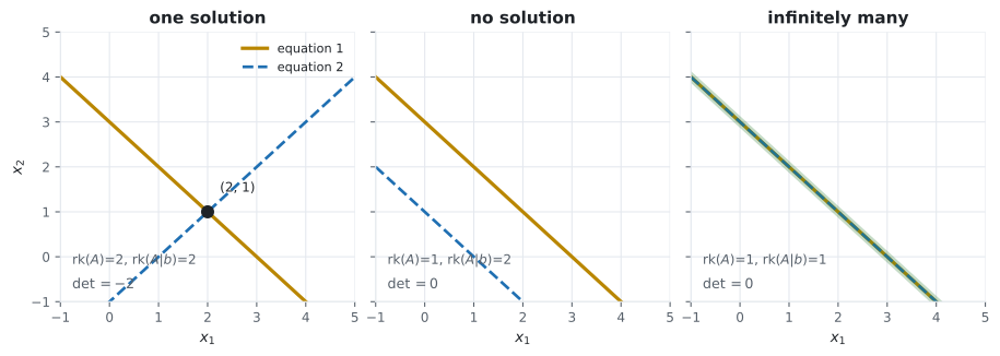
Section titled “Exactly three outcomes”For a real-valued system there are only three possibilities: no solution, exactly one, or infinitely many. Nothing else can happen — you cannot have exactly two.
With two unknowns, each equation is a line in the -plane, and a solution must lie on all lines at once, so the solution set is their intersection:
| lines | intersection | solutions |
|---|---|---|
| cross at a point | a point | exactly one |
| parallel, distinct | empty | none |
| identical | the whole line | infinitely many |
With three unknowns each equation is a plane, and intersecting planes gives a plane, a line, a point, or nothing — the same three outcomes, one dimension up. The book states this generalisation explicitly and it keeps holding: in each equation is a hyperplane, and the solution set is an intersection of hyperplanes.
Why “exactly two” is impossible is worth seeing, because it is the first place the structure shows. Suppose and are both solutions. Then for any ,
so the whole line through them is made of solutions. Two solutions therefore force infinitely many. Linearity does not permit a finite crowd.
Worked example by hand
Section titled “Worked example by hand”Back to the tables and chairs:
From the second equation, , so . Substituting into the first:
Two-thirds of a table is not a useful production plan, which is a nice reminder that “solvable” and “meaningful” are different questions — but it is the unique solution.
Now the book’s own geometric example, and every step by hand:
Adding the two equations kills outright: , so . Back-substituting into the first, , so . The solution is — exactly the point the book’s Figure 2.3 marks.
And a system of each of the three kinds, checked in full:
| system | manipulation | outcome |
|---|---|---|
| , | add: | one: |
| , | subtract: | none — a contradiction |
| , | halve the second: identical | infinitely many: |
The middle row is the one to remember. Elimination did not fail or get stuck; it produced the perfectly well-formed statement , which is false. Inconsistency shows up as a false arithmetic claim, and that is precisely what §2.3’s elimination procedure is built to surface.
See it move
Section titled “See it move”Two lines. The amber one is fixed; the blue one sweeps through all three regimes. The white dot marks the solution when it exists — watch it fly off to infinity as the lines become parallel, then the lines merge.
Watch the det readout in the corner. It slides towards zero as the lines become parallel and hits
zero exactly when the regime changes. That number is the determinant (§4.1), and it is the single
quantity deciding which of the three cases you are in — the sketch is showing you §4.1’s punchline
two chapters early.
And the same system, solved step by step
Section titled “And the same system, solved step by step”Elimination on the workshop system, one row operation per frame. The pivot is ringed; the row being rewritten is amber, and the row doing the rewriting is blue.
Two pivots for two unknowns means exactly one solution, and the reduced form puts it in the right-hand column.
Two pivots for two unknowns — that is what “exactly one solution” looks like mechanically, and §2.3 turns the observation into the general procedure.
From scratch
Section titled “From scratch”import numpy as np
# ---- the workshop system -------------------------------------------------
# 4*x1 + 1*x2 = 5 (wood)
# 2*x1 + 2*x2 = 6 (labour)
A = np.array([[4.0, 1.0],
[2.0, 2.0]])
b = np.array([5.0, 6.0])
x = np.linalg.solve(A, b)
print("tables x1 =", round(x[0], 4), " chairs x2 =", round(x[1], 4))
print("check A @ x =", A @ x)
print("determinant :", np.linalg.det(A))
# ---- the columns view: x scales the columns ------------------------------
c1, c2 = A[:, 0], A[:, 1]
print("x1*c1 + x2*c2 =", x[0] * c1 + x[1] * c2, " == b:", np.allclose(x[0] * c1 + x[1] * c2, b))
# ---- the book's Figure 2.3 system ---------------------------------------
A2 = np.array([[4.0, 4.0], [2.0, -4.0]])
b2 = np.array([5.0, 1.0])
print("\nFigure 2.3 solution:", np.linalg.solve(A2, b2))
# ---- the three regimes, detected rather than guessed --------------------
def classify(A, b):
"""Rank of A versus rank of the augmented matrix decides the regime."""
rank_A = np.linalg.matrix_rank(A)
rank_Ab = np.linalg.matrix_rank(np.c_[A, b])
n = A.shape[1]
if rank_A < rank_Ab:
return "no solution"
return "exactly one" if rank_A == n else f"infinitely many ({n - rank_A} free)"
cases = {
"crossing": (np.array([[1.0, 1.0], [1.0, -1.0]]), np.array([3.0, 1.0])),
"parallel": (np.array([[1.0, 1.0], [1.0, 1.0]]), np.array([3.0, 1.0])),
"identical": (np.array([[1.0, 1.0], [2.0, 2.0]]), np.array([3.0, 6.0])),
}
print()
for name, (M, v) in cases.items():
print(f"{name:10s} rk(A)={np.linalg.matrix_rank(M)} "
f"rk(A|b)={np.linalg.matrix_rank(np.c_[M, v])} -> {classify(M, v)}")
# ---- what solve does when there is not exactly one solution -------------
try:
np.linalg.solve(cases["parallel"][0], cases["parallel"][1])
except np.linalg.LinAlgError as e:
print("\nsolve on the parallel case:", e)tables x1 = 0.6667 chairs x2 = 2.3333
check A @ x = [5. 6.]
determinant : 6.0
x1*c1 + x2*c2 = [5. 6.] == b: True
Figure 2.3 solution: [1. 0.25]
crossing rk(A)=2 rk(A|b)=2 -> exactly one
parallel rk(A)=1 rk(A|b)=2 -> no solution
identical rk(A)=1 rk(A|b)=1 -> infinitely many (1 free)
solve on the parallel case: Singular matrixThe classify function is worth more than it looks. Comparing with
decides the regime without trying to solve anything
— and that is exactly the criterion §2.6 states as a property of rank. The three-line function is
that theorem, executed.
On real data
Section titled “On real data”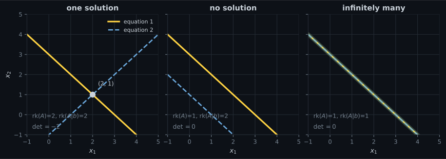
Reading the plot
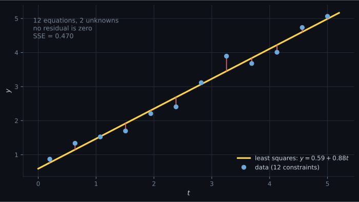
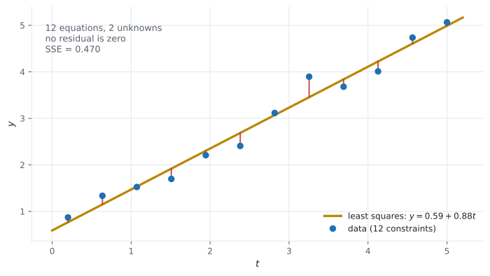
Section titled “Reading the plot”The second figure is the case machine learning actually lives in. Twelve data points give twelve equations in two unknowns (slope and intercept). The system is overdetermined, and unless the points happen to be exactly collinear there is no solution at all — the middle panel of the first figure, in twelve dimensions.
So the correct response is not to hunt for a better solver. It is to change the question: instead of “which line passes through every point”, ask “which line minimises the total squared miss”. That is least squares, it always has an answer, and Chapter 9 derives it. §3.8 then shows the answer is a solution to a related system — the normal equations — so the machinery of this chapter is not abandoned, it is redeployed.
Pitfalls
Section titled “Pitfalls”Compare
Section titled “Compare”| situation | shape | typically | what to do |
|---|---|---|---|
| , independent rows | square | exactly one solution | np.linalg.solve |
| (overdetermined) | tall | no exact solution | least squares — lstsq, Chapter 9 |
| (underdetermined) | wide | infinitely many | add constraints, or take the minimum-norm solution via pinv |
| , dependent rows | square, singular | none or infinitely many | check |
-
A system of linear equations has two distinct solutions. How many does it have in total?
Any weighted average of two solutions is also a solution, because the map is linear. So two solutions force the whole line through them to be solutions — a finite crowd larger than one is impossible.
pch.quizShowAnswer
B — Infinitely many — Any weighted average of two solutions is also a solution, because the map is linear. So two solutions force the whole line through them to be solutions — a finite crowd larger than one is impossible.
-
In the columns view, what is the equation Ax = b actually asking?
The unknowns scale the columns. That turns solvability into a question about reach — is b inside what the columns can build — which sections 2.5, 2.6 and 2.7 name the span, the rank and the image.
pch.quizShowAnswer
B — Whether b can be built as a weighted combination of the columns of A, and with which weights — The unknowns scale the columns. That turns solvability into a question about reach — is b inside what the columns can build — which sections 2.5, 2.6 and 2.7 name the span, the rank and the image.
-
You get LinAlgError Singular matrix. What do you know?
Both the parallel and the identical cases are singular. Distinguishing them needs the rank of A compared against the rank of the augmented matrix.
pch.quizShowAnswer
C — There is not exactly one solution — it could be none or infinitely many — Both the parallel and the identical cases are singular. Distinguishing them needs the rank of A compared against the rank of the augmented matrix.
-
Twelve data points, a straight-line model with two parameters. What is the situation?
Each point demands the line pass through it, so it is overdetermined. Unless the points are exactly collinear no line satisfies all twelve, which is why the answer is least squares rather than a solver.
pch.quizShowAnswer
A — Twelve equations in two unknowns, almost certainly with no exact solution — Each point demands the line pass through it, so it is overdetermined. Unless the points are exactly collinear no line satisfies all twelve, which is why the answer is least squares rather than a solver.
🧪 Try It Yourself
Section titled “🧪 Try It Yourself”Exercise 1 – Solve a 2×2 system
Section titled “Exercise 1 – Solve a 2×2 system”Exercise 2 – The unknowns scale the columns
Section titled “Exercise 2 – The unknowns scale the columns”Exercise 3 – Classify a system without solving it
Section titled “Exercise 3 – Classify a system without solving it”Exercise 4 – Two solutions force infinitely many
Section titled “Exercise 4 – Two solutions force infinitely many”Exercise 5 – Overdetermined, so least squares
Section titled “Exercise 5 – Overdetermined, so least squares”Recall card
Section titled “Recall card”- A system of linear equations asks for values satisfying several linear constraints at once, and every unknown appears to the first power only.
- Linearity is a condition on the unknowns, not the data — coefficients may be arbitrarily nonlinear functions of the inputs, which is the loophole feature maps exploit.
- The unknowns scale the columns, so solving asks whether b is reachable as a weighted combination of the columns of A.
- There are exactly three outcomes — none, one, or infinitely many — because two distinct solutions force the whole line through them to be solutions.
- Geometrically the solution set is an intersection: of lines in two variables, planes in three, hyperplanes in general.
- Inconsistency surfaces as a false arithmetic statement like , rather than as a stuck computation.
Singular matrixmeans “not exactly one”, not “none” — the parallel and identical cases are both singular.- Comparing the rank of A with the rank of the augmented matrix decides the regime without solving anything.
- Overdetermined systems are the normal case in machine learning, and the response is least squares rather than a better solver.
Next: compress the whole system into one object — the matrix — which both stores data and transforms it.
pch.coffeeTagline
pch.coffeeCtapch.feedbackHeading
pch.feedbackSubheading