Overfitting in Linear Regression

Page 902 produced a formula that works for any $K$ . This page asks what happens as $K$ grows, and the answer is Chapter 8’s §8.3.3 arriving with concrete numbers attached — “we suffer from overfitting”.

Three results, all measured: the training error cannot rise, which is why it cannot be trusted; the estimator stops being unique at $M \geqslant N$ ; and the degree the book picks is one draw of a random experiment, winning only $46.1\%$ of repeats.

What you’ll learn

Equation 9.23, the RMSE — and the two reasons the book prefers it, both checkable.
Why “the training error never increases” is a theorem rather than an observation — verified across nine steps, zero increases.
The book’s search bound $0 \leqslant M \leqslant N-1$ , and what happens past it: measured, a null space of dimension $1$ and infinitely many estimators fitting equally well.
Figure 9.6 reproduced: the test error bottoms out at $M = 4$ at $0.324947$ , then reaches $\mathbf{100.850623}$ at $M = 9$ .
At $M = N - 1 = 9$ : training RMSE $\mathbf{6.506\times10^{-11}}$ — the curve passes through every point — and the worst test error on the page.
How stable that conclusion is. Repeated on $2000$ fresh draws, $M = 4$ wins $46.1\%$ , $M = 6$ wins $20.8\%$ , $M = 1$ wins $11.3\%$ .

Intuition: the exam you wrote yourself

The training error can never rise as you add capacity, and the reason is set inclusion rather than statistics. Every degree-4 polynomial is also a degree-5 polynomial — set $\theta_5 = 0$ . So the degree-5 class contains everything the degree-4 class could do, and its best member cannot be worse.

That single fact is why a falling training curve carries no information. It would fall for a model that generalised perfectly and for one that memorised the data, and by $M = N-1$ it reaches zero — a polynomial through $N$ points exists and is unique, so the fit is exact and says nothing at all.

What it does leave behind is a fingerprint. Interpolating $N$ scattered points requires violent oscillation between them, and violent oscillation requires large coefficients. The parameter norm is the one warning visible without a test set — which is precisely the handle §9.2.3 grabs.

diagram Why the training curve is useless and what replaces it mermaid

  flowchart TD
  A["degree M class contains degree M-1 class
(set theta_M = 0)"]
  A --> B["best fit cannot get worse
THEOREM, not observation"]
  B --> C["training RMSE monotone
measured: 9 steps, 0 increases"]
  C --> D["at M = N-1 it hits 0
measured 6.5e-11"]
  D --> E["so it carries NO information
about generalization"]
  E --> F["a held-out set, Eq 9.23
test RMSE bottoms at M = 4"]
  E --> G["or the parameter norm
0.99 at M=4, 4.20 at M=9"]
  G -.->|"Section 9.2.3 acts on this"| H["a prior on theta"]

§9.2.2 Measuring the error

The negative log-likelihood works, but since “the noise parameter $\sigma^2$ is not a free model parameter, we can ignore the scaling by $1/\sigma^2$ ”, leaving $\lVert\mathbf{y} - \boldsymbol\Phi\boldsymbol\theta\rVert^2$ . The book then prefers the root mean square error, Equation 9.23:

\sqrt{\frac{1}{N}\lVert\mathbf{y} - \boldsymbol\Phi\boldsymbol\theta\rVert^2} = \sqrt{\frac{1}{N}\sum_{n=1}^{N}\left(y_n - \phi^\top(x_n)\boldsymbol\theta\right)^2}

for two stated reasons: it “(a) allows us to compare errors of datasets with different sizes” and “(b) has the same scale and the same units as the observed function values $y_n$ .”

The book’s own illustration: mapping post-codes to house prices in EUR gives an RMSE in EUR, while the squared error is in EUR², and including $\sigma^2$ leaves “a unitless objective”.

Scale every target by $c$ and refit:

scale $c$ on $y$	RMSE	RMSE / $c$	NLL	NLL / $c$
$1.0$	$0.270626$	$\mathbf{0.270626}$	$9.154787$	$9.154787$
$10.0$	$2.706257$	$\mathbf{0.270626}$	$915.478700$	$91.547870$
$1000.0$	$270.625749$	$\mathbf{0.270626}$	$9154787.004056$	$9154.787004$

The RMSE scales exactly with $c$ — divide it out and you recover the identical number, which is what “has the units of $y$ ” means operationally. The negative log-likelihood scales with $c^2$ and carries $\sigma^2$ inside it, so dividing by $c$ recovers nothing. It is not in the units of $y$ at all.

The training error cannot rise

Note that the training error never increases when the degree of the polynomial increases.

$M-1 \to M$	change in training RMSE
$0 \to 1$	$-2.344\times10^{-1}$
$1 \to 2$	$-1.536\times10^{-1}$
$2 \to 3$	$-6.551\times10^{-2}$
$3 \to 4$	$-2.539\times10^{-1}$
$4 \to 5$	$-5.028\times10^{-4}$
$5 \to 6$	$-6.254\times10^{-2}$
$6 \to 7$	$-1.511\times10^{-2}$
$7 \to 8$	$-3.158\times10^{-2}$
$8 \to 9$	$-1.609\times10^{-1}$

Every step negative. This is a theorem, not a measurement: the degree- $M$ class contains the degree- $(M{-}1)$ class as the subset with $\theta_M = 0$ , so its minimum over a larger set cannot be larger. Note $4 \to 5$ at $-5.0\times10^{-4}$ — nearly flat, because the extra term buys almost nothing — but still not positive.

Choosing the degree, and the bound

For model selection “we can use the RMSE (or the negative log-likelihood) to determine the best degree of the polynomial”, and since the degree is a natural number, “we can perform a brute-force search and enumerate all (reasonable) values of $M$ .”

For a training set of size $N$ it is sufficient to test $0 \leqslant M \leqslant N-1$ . For $M < N$ , the maximum likelihood estimator is unique. For $M \geqslant N$ , we have more parameters than data points, and would need to solve an underdetermined system of linear equations so that there are infinitely many possible maximum likelihood estimators.

At $M = 10$ with $N = 10$ : $\mathrm{rk}(\boldsymbol\Phi) = 10$ , $K = 11$ , so the null space has dimension $\mathbf{1}$ . Add any multiple of a null vector and the training fit is unchanged:

estimator	training RMSE	$\lVert\boldsymbol\theta\rVert$
minimum-norm (`lstsq`)	$5.145\times10^{-10}$	$3.441536$
$+\ 1.0 \times$ null vector	$4.678\times10^{-10}$	$3.583876$
$+\ 50.0 \times$ null vector	$1.839\times10^{-9}$	$50.118302$
$+\ 5000.0 \times$ null vector	$2.342\times10^{-7}$	$5000.001184$

All four fit the training data equally well and their norms differ by three orders of magnitude. “The maximum likelihood estimator” stops being a definite article. np.linalg.lstsq silently returns the minimum-norm member — a reasonable choice, and not one the likelihood made.

Figure 9.6, reproduced

The book’s setup: $N = 10$ training points with $x_n \sim \mathcal{U}[-5,5]$ and $y_n = -\sin(x_n/5) + \cos(x_n) + \epsilon$ , $\epsilon \sim \mathcal{N}(0, 0.2^2)$ , against a test set of “200 data points … a linear grid of 200 points in the interval $[-5,5]$ .”

$M$	$K = M{+}1$	training RMSE	test RMSE	$\lVert\boldsymbol\theta\rVert$
$0$	$1$	$0.977999$	$0.893710$	$0.2135$
$1$	$2$	$0.743590$	$0.745097$	$0.2150$
$2$	$3$	$0.590009$	$0.688459$	$0.5211$
$3$	$4$	$0.524501$	$0.785402$	$0.7584$
$\mathbf{4}$	$5$	$0.270626$	$\mathbf{0.324947}$	$0.9904$
$5$	$6$	$0.270123$	$0.333082$	$1.0069$
$6$	$7$	$0.207586$	$0.473424$	$1.1985$
$7$	$8$	$0.192473$	$0.664497$	$0.9769$
$8$	$9$	$0.160893$	$7.420601$	$1.1314$
$9$	$10$	$\mathbf{6.506\times10^{-11}}$	$\mathbf{100.850623}$	$4.2030$

Best test RMSE at $M = 4$ — the book’s answer, reproduced. Its description of the shape holds too: the test error “is relatively low and stays relatively constant up to degree 5” ( $0.324947$ then $0.333082$ ), and “from degree 6 onward the test error increases significantly” ( $0.473$ , $0.664$ , $7.42$ , $100.85$ ).

One honest deviation. Between $M = 2$ and $M = 3$ the test error goes up, $0.688459 \to 0.785402$ , before the real minimum at $M = 4$ . The test curve is not U-shaped; it is noisy and roughly U-shaped, and a search that stopped at the first increase would have chosen $M = 2$ .

	$M = 8$	$M = 9 = N-1$
training RMSE	$1.609\times10^{-1}$	$\mathbf{6.506\times10^{-11}}$
test RMSE	$7.4206$	$\mathbf{100.8506}$
$\lVert\boldsymbol\theta\rVert$	$1.1314$	$4.2030$

“In the extreme case of $M = N - 1 = 9$ , the function will pass through every single data point. However, these high-degree polynomials oscillate wildly.” Perfect interpolation and the worst generalization on the page, in the same column.

How much does Figure 9.6 actually tell you?

Figure 9.6 is a single draw of a random experiment. The obvious question — would another draw give the same answer? — is not one the book asks.

$M$	times chosen	share
$0$	$65$	$3.2\%$
$1$	$226$	$11.3\%$
$2$	$153$	$7.6\%$
$3$	$1$	$0.1\%$
$\mathbf{4}$	$\mathbf{921}$	$\mathbf{46.1\%}$
$5$	$152$	$7.6\%$
$6$	$417$	$\mathbf{20.8\%}$
$7$	$56$	$2.8\%$
$8$	$9$	$0.4\%$
$9$	$0$	$0.0\%$

Median best test RMSE across draws: $0.418686$ .

$M = 4$ is the right answer — and it wins less than half the time. $M = 6$ takes $20.8\%$ , and $M = 1$ takes $11.3\%$ . Two things follow.

The book’s conclusion is correct as a modal statement and would be overclaimed as a determination. And $N = 10$ is simply too small for the selection to be stable — which is the same boundary page 808’s standard-error measurement kept arriving at from the cross-validation side.

Note also $M = 3$ at $0.1\%$ : the strange bump in the single-draw table was not a fluke of that draw. Degree 3 is a genuinely poor choice for this function, sitting between the useful low degrees and the degree-4 fit that finally captures the cosine.

Worked example by hand

Why does a richer model class have a smaller training error? Prove it, then check the one case where equality can happen.

Step 1: state the claim. Let $\mathcal{F}_M$ be the polynomials of degree at most $M$ , and $E(M) := \min_{f \in \mathcal{F}_M}\sum_n (y_n - f(x_n))^2$ . Claim: $E(M) \leqslant E(M-1)$ .

Step 2: the containment. Any $f \in \mathcal{F}_{M-1}$ can be written in $\mathcal{F}_M$ by taking $\theta_M = 0$ . So $\mathcal{F}_{M-1} \subseteq \mathcal{F}_M$ .

Step 3: a minimum over a larger set is no larger. If $S \subseteq T$ then $\min_T g \leqslant \min_S g$ , because every candidate in $S$ is also a candidate in $T$ . Hence

E(M) = \min_{\mathcal{F}_M} \leqslant \min_{\mathcal{F}_{M-1}} = E(M-1)

No property of polynomials was used — only nesting. The same argument covers adding any feature to any linear model.

Step 4: when is it an equality? Exactly when the extra column buys nothing, i.e. when the optimal $\theta_M$ is already zero — meaning $\phi_M$ is orthogonal to the residual of the smaller fit. Measured above at $4 \to 5$ : a change of $-5.028\times10^{-4}$ , nearly but not quite equality.

Step 5: the endpoint. At $M = N-1$ there is a unique polynomial of degree $\leqslant N-1$ through $N$ distinct points, so the residual is exactly zero and $E(N-1) = 0$ . Measured: $6.506\times10^{-11}$ , which is zero to conditioning. No further degree can improve on zero, so the bound $M \leqslant N-1$ is not conservatism — it is where the training criterion runs out entirely.

Step 6: read the consequence. A quantity guaranteed to move one way regardless of the truth carries no information about the truth. That is the whole argument for a held-out set — and, from the other direction, for the prior §9.2.3 is about to introduce.

See it move

sketch Watch the training error fall while the fit gets worse p5.js

Polynomial fits to ten noisy points, degree 0 through 10. Drag the degree and watch the training RMSE fall monotonically while the test RMSE bottoms out and then explodes. Drag the noise level to see how quickly the best degree moves.

From scratch

overfitting.py

import numpy as np
 
SIG = 0.2
NTR = 10
 
def truth(x):
    """The book's generating function, Example 9.5."""
    return -np.sin(x / 5) + np.cos(x)
 
def design(x, M):
    return np.vander(np.asarray(x, float), M + 1, increasing=True)
 
def train_set(seed):
    rng = np.random.default_rng(seed)
    x = np.sort(rng.uniform(-5, 5, NTR))
    return x, truth(x) + SIG * rng.standard_normal(NTR)
 
def rmse(a, b):
    return float(np.sqrt(np.mean((a - b) ** 2)))       # Equation 9.23
 
# the book's test set: "a linear grid of 200 points in the interval [-5, 5]"
xte = np.linspace(-5, 5, 200)
yte = truth(xte) + SIG * np.random.default_rng(1234).standard_normal(200)
 
# --- Figure 9.6 ---------------------------------------------------------
print("=== 1. Figure 9.6 reproduced: training and test RMSE ===")
x, y = train_set(4)
print(f"{'M':>4} {'K = M+1':>8} {'training RMSE':>15} {'test RMSE':>12} "
      f"{'||theta||':>13}")
tr, te = [], []
for M in range(10):
    P = design(x, M)
    th = np.linalg.lstsq(P, y, rcond=None)[0]
    a, b = rmse(y, P @ th), rmse(yte, design(xte, M) @ th)
    tr.append(a); te.append(b)
    print(f"{M:>4} {M+1:>8} {a:>15.6f} {b:>12.6f} "
          f"{np.linalg.norm(th):>13.4f}")
print(f"\nbest test RMSE at M = {int(np.argmin(te))} ({min(te):.6f})")
 
# --- the training error never rises -------------------------------------
print("\n=== 2. the training error never increases with M ===")
print(f"{'M-1 -> M':>10} {'change in training RMSE':>26}")
for M in range(1, 10):
    print(f"{M-1:>4} -> {M:<3} {tr[M]-tr[M-1]:>26.3e}")
print(f"steps where it went UP: "
      f"{sum(1 for M in range(1,10) if tr[M] > tr[M-1])}")
print("a richer class contains the poorer one, so its best fit cannot be")
print("worse ON THE TRAINING SET. A theorem, not an observation.")
 
# --- the extreme case ----------------------------------------------------
print("\n=== 3. at M = N - 1 the curve passes through every point ===")
for M in (8, 9):
    P = design(x, M)
    th = np.linalg.lstsq(P, y, rcond=None)[0]
    print(f"M = {M}: training RMSE {rmse(y, P @ th):.3e}   "
          f"test RMSE {rmse(yte, design(xte, M) @ th):>12.4f}   "
          f"||theta|| {np.linalg.norm(th):.4f}")
 
# --- past the bound, the estimator is not unique ------------------------
print("\n=== 4. for M >= N there are INFINITELY many estimators ===")
M = 10
P = design(x, M)
th_min = np.linalg.lstsq(P, y, rcond=None)[0]
ns = np.linalg.svd(P)[2][int(np.linalg.matrix_rank(P)):]
print(f"M = {M}, K = {P.shape[1]}, N = {NTR}, "
      f"rk(Phi) = {int(np.linalg.matrix_rank(P))}")
print(f"dimension of the null space of Phi: {ns.shape[0]}")
print(f"\n{'estimator':>26} {'training RMSE':>15} {'||theta||':>14}")
print(f"{'minimum-norm (lstsq)':>26} {rmse(y, P @ th_min):>15.3e} "
      f"{np.linalg.norm(th_min):>14.6f}")
for c in (1.0, 50.0, 5000.0):
    alt = th_min + c * ns[0]
    print(f"{'  + ' + str(c) + ' * null vector':>26} "
          f"{rmse(y, P @ alt):>15.3e} {np.linalg.norm(alt):>14.6f}")
print("all of them fit the training data equally well.")
 
# --- the RMSE has the units of y ----------------------------------------
print("\n=== 5. RMSE has the units of y; the NLL does not ===")
P = design(x, 4)
print(f"{'scale c on y':>14} {'RMSE':>14} {'RMSE / c':>14} "
      f"{'NLL':>16} {'NLL / c':>16}")
for c in (1.0, 10.0, 1000.0):
    yc = c * y
    r = yc - P @ np.linalg.lstsq(P, yc, rcond=None)[0]
    rc = float(np.sqrt(np.mean(r ** 2)))
    nll = float(r @ r / (2 * SIG ** 2))
    print(f"{c:>14.1f} {rc:>14.6f} {rc/c:>14.6f} {nll:>16.6f} "
          f"{nll/c:>16.6f}")
print("RMSE scales exactly with c; the NLL scales with c^2 and carries")
print("sigma^2, so it is not in the units of y at all.")
 
# --- how stable is 'the best degree is 4'? ------------------------------
print("\n=== 6. how stable is 'the best degree is 4'? ===")
counts = np.zeros(10, dtype=int)
best_te = []
for s in range(2000):
    xs, ys = train_set(10_000 + s)
    scores = [rmse(yte, design(xte, M)
                   @ np.linalg.lstsq(design(xs, M), ys, rcond=None)[0])
              for M in range(10)]
    k = int(np.argmin(scores))
    counts[k] += 1
    best_te.append(scores[k])
print(f"{'M':>4} {'chosen':>9} {'share':>9}")
for M in range(10):
    print(f"{M:>4} {counts[M]:>9} {counts[M]/2000:>8.1%}")
print(f"\nmedian best test RMSE: {np.median(best_te):.6f}")
print(f"the modal choice is M = {int(np.argmax(counts))}")
print("Figure 9.6 is one draw of a random experiment, and the degree it")
print("singles out moves with the draw.")

text

=== 1. Figure 9.6 reproduced: training and test RMSE ===
   M  K = M+1   training RMSE    test RMSE     ||theta||
   0        1        0.977999     0.893710        0.2135
   1        2        0.743590     0.745097        0.2150
   2        3        0.590009     0.688459        0.5211
   3        4        0.524501     0.785402        0.7584
   4        5        0.270626     0.324947        0.9904
   5        6        0.270123     0.333082        1.0069
   6        7        0.207586     0.473424        1.1985
   7        8        0.192473     0.664497        0.9769
   8        9        0.160893     7.420601        1.1314
   9       10        0.000000   100.850623        4.2030
 
best test RMSE at M = 4 (0.324947)
 
=== 2. the training error never increases with M ===
  M-1 -> M    change in training RMSE
   0 -> 1                   -2.344e-01
   1 -> 2                   -1.536e-01
   2 -> 3                   -6.551e-02
   3 -> 4                   -2.539e-01
   4 -> 5                   -5.028e-04
   5 -> 6                   -6.254e-02
   6 -> 7                   -1.511e-02
   7 -> 8                   -3.158e-02
   8 -> 9                   -1.609e-01
steps where it went UP: 0
a richer class contains the poorer one, so its best fit cannot be
worse ON THE TRAINING SET. A theorem, not an observation.
 
=== 3. at M = N - 1 the curve passes through every point ===
M = 8: training RMSE 1.609e-01   test RMSE       7.4206   ||theta|| 1.1314
M = 9: training RMSE 6.506e-11   test RMSE     100.8506   ||theta|| 4.2030
 
=== 4. for M >= N there are INFINITELY many estimators ===
M = 10, K = 11, N = 10, rk(Phi) = 10
dimension of the null space of Phi: 1
 
                 estimator   training RMSE      ||theta||
      minimum-norm (lstsq)       5.145e-10       3.441536
       + 1.0 * null vector       4.678e-10       3.583876
      + 50.0 * null vector       1.839e-09      50.118302
    + 5000.0 * null vector       2.342e-07    5000.001184
all of them fit the training data equally well.
 
=== 5. RMSE has the units of y; the NLL does not ===
  scale c on y           RMSE       RMSE / c              NLL          NLL / c
           1.0       0.270626       0.270626         9.154787         9.154787
          10.0       2.706257       0.270626       915.478700        91.547870
        1000.0     270.625749       0.270626   9154787.004056      9154.787004
RMSE scales exactly with c; the NLL scales with c^2 and carries
sigma^2, so it is not in the units of y at all.
 
=== 6. how stable is 'the best degree is 4'? ===
   M    chosen     share
   0        65     3.2%
   1       226    11.3%
   2       153     7.6%
   3         1     0.1%
   4       921    46.1%
   5       152     7.6%
   6       417    20.8%
   7        56     2.8%
   8         9     0.4%
   9         0     0.0%
 
median best test RMSE: 0.418686
the modal choice is M = 4
Figure 9.6 is one draw of a random experiment, and the degree it
singles out moves with the draw.

On real data

Six panels showing polynomial fits of degree 0, 1, 3, 4, 6 and 9 to the same ten points, with the generating function dashed behind each. The last panel oscillates violently between the data points. — Read the two numbers in each panel together. Training error falls at every step while test error bottoms out at M = 4 with 0.324947 and then leaves — reaching 100.850623 at M = 9, exactly where the fit becomes perfect at 6.5e-11.

Left, two curves on a log scale against polynomial degree: a training curve falling monotonically off the bottom of the plot and a test curve dipping at degree 4 then rising steeply. Right, the parameter norm against degree, rising sharply at the end. — Nine steps, zero increases — a theorem from set inclusion rather than an empirical pattern. The test curve bottoms at M = 4 as the book reports, with one honest deviation: it bumps upward between M = 2 and M = 3 before the real minimum.

Left, a bar chart of how often each degree wins across two thousand repeats, with degree 4 tallest at just under half and degree 6 second. Right, four polynomial curves of degree 10 all passing through the same ten points while differing wildly between them. — Degree 4 is the modal answer and wins only 46.1 percent of two thousand fresh draws; degree 6 takes 20.8 percent. On the right, the null space has dimension one, so adding any multiple of a null vector gives a different parameter vector that fits the training data just as well.

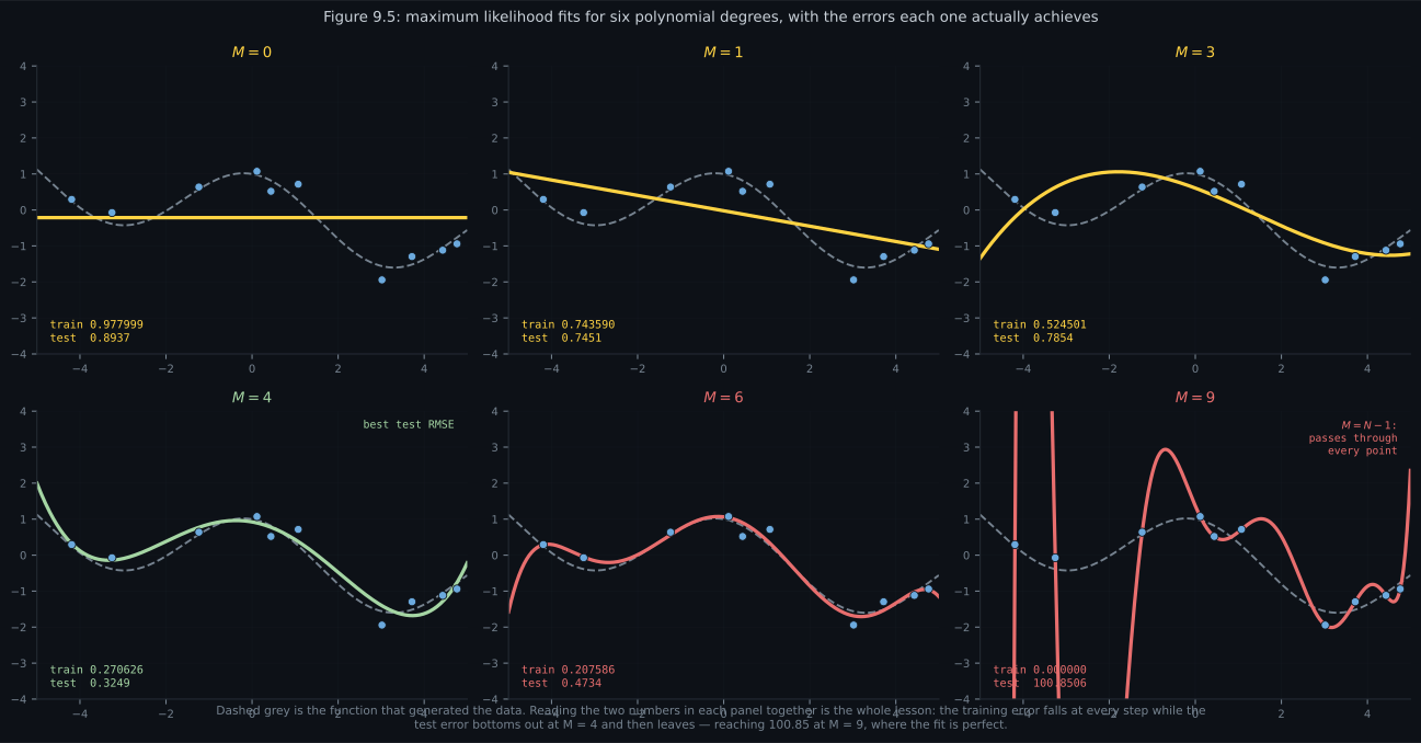
Reading the plot

The first figure is Figure 9.5 with the numbers the book leaves in its prose. The dashed grey curve is the generating function; each panel’s two figures are its training and test RMSE. Reading down them is the entire lesson: training goes $0.978 \to 0.744 \to 0.525 \to 0.271 \to 0.208 \to 6.5\times10^{-11}$ , never once rising, while test goes $0.894 \to 0.745 \to 0.785 \to 0.325 \to 0.473 \to 100.85$ .

The $M = 9$ panel is the one to sit with. The curve passes through all ten points. Its training error is $6.5\times10^{-11}$ — zero, to conditioning. And its test error is $100.85$ , the worst on the page by a factor of thirteen. A perfect fit and no knowledge, in the same object.

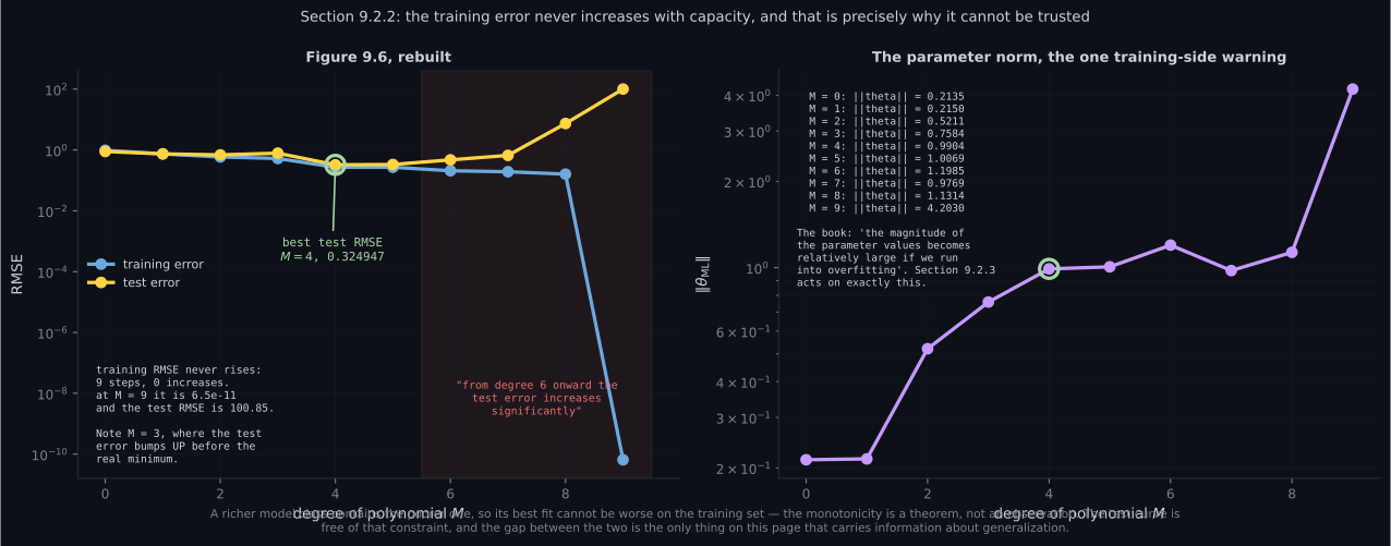
The second figure separates a theorem from an observation. The training curve’s monotonicity is not a pattern that happened to hold on this data. Every degree- $M$ polynomial is a degree- $(M{+}1)$ polynomial with a zero coefficient, so the larger class’s minimum cannot exceed the smaller’s. It would fall identically for a model that generalises and one that memorises, which is exactly why it carries no information.

The step $4 \to 5$ is the interesting one: $-5.028\times10^{-4}$ . Almost flat — the fifth-degree term buys essentially nothing — but still negative, because the theorem does not permit otherwise.

The right panel is what the training side can tell you. $\lVert\boldsymbol\theta\rVert$ climbs from $0.9904$ at the good degree to $4.2030$ at $M = 9$ . The book’s own sentence in §9.2.3 is “the magnitude of the parameter values becomes relatively large if we run into overfitting”, and it is the entire motivation for the prior on the next page. Interpolating scattered points requires oscillation, and oscillation requires large coefficients — so the fingerprint is visible without a test set.

And one honest deviation from the book’s description. The test error goes up from $M = 2$ to $M = 3$ — $0.688459$ to $0.785402$ — before the real minimum at $M = 4$ . The book describes the curve as initially decreasing; on this draw it is noisy and roughly U-shaped, and a search that stopped at the first increase would have chosen $M = 2$ and been wrong.

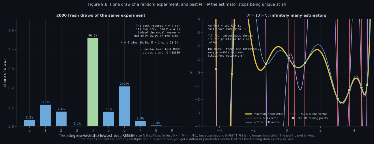
The third figure asks a question the book does not, and the answer changes how much Figure 9.6 is worth. Repeat the whole experiment — fresh $x$ , fresh noise, same $N = 10$ , same test grid — two thousand times, and record which degree wins. $M = 4$ wins $921$ times: $46.1\%$ . $M = 6$ wins $20.8\%$ . $M = 1$ wins $11.3\%$ .

So the book’s conclusion is right — $M = 4$ is the modal answer and the median best test RMSE is $0.418686$ — and it is right the way a coin that lands heads $46\%$ of the time is a reasonable bet, not the way a theorem is right. With ten training points the selection is simply not stable, which is the same $N$ -is-too-small boundary page 808 measured from the cross-validation side and page 902 measured in the noise-variance bias.

Note $M = 3$ winning once in two thousand draws. The bump in the single-draw table was not an accident of that draw — degree 3 is genuinely poor here, caught between the low degrees that at least capture the trend and the degree-4 fit that finally accommodates the cosine.

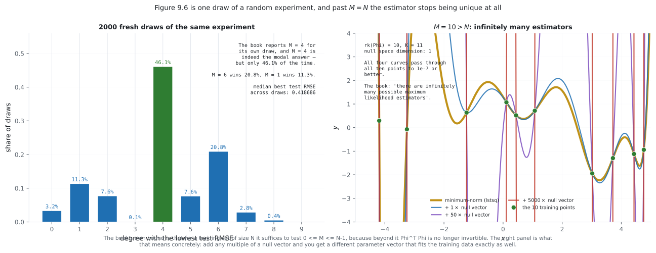
The right panel is the bound $M \leqslant N-1$ made visible. At $M = 10$ the null space has dimension one, and the four plotted curves are $\boldsymbol\theta_{\text{min}} + c\,\mathbf{n}$ for $c \in \{0, 1, 50, 5000\}$ . They all pass through all ten training points, and their norms run from $3.44$ to $5000.00$ . “The maximum likelihood estimator” is no longer a definite article. np.linalg.lstsq returns the minimum-norm one — a sensible convention, but a convention, not something the likelihood determined.

Compare

	training error	test error
direction as $M$ grows	monotone non-increasing, guaranteed	free to do anything
at $M = N-1$	exactly $0$ (measured $6.5\times10^{-11}$ )	worst on the page, $100.85$
measured here	$0.978 \to 6.5\times10^{-11}$	$0.894 \to 0.325 \to 100.85$
detects underfitting	yes	yes
detects overfitting	no	yes
needs held-out data	no	yes

	RMSE, Eq 9.23	squared error	negative log-likelihood
units	same as $y$ (EUR)	$y$ squared (EUR²)	unitless
scaling $y$ by $c$	$\times c$	$\times c^2$	$\times c^2$
comparable across $N$	yes	no	no
contains $\sigma^2$	no	no	yes

	$M < N$	$M \geqslant N$
$\mathrm{rk}(\boldsymbol\Phi)$ vs $K$	$=K$	$<K$
$\boldsymbol\Phi^\top\boldsymbol\Phi$	invertible	singular
estimators	exactly one	infinitely many
what `lstsq` returns	the estimator	the minimum-norm one, by convention
the book’s advice	search $0 \leqslant M \leqslant N-1$	do not go here

pch.quizTag Do you know what the training curve is worth?

The book says the training error never increases as the polynomial degree grows. Why is that guaranteed rather than merely observed?

pch.quizShowAnswer

B — Because the degree-M class contains the degree-(M-1) class as the subset with the top coefficient zero, so its minimum cannot be larger — No property of polynomials is used — only nesting, so the same argument covers adding any feature to any linear model. Measured across nine steps: zero increases, including the near-flat 4 to 5 step at -5.028e-4. And a quantity guaranteed to move one way regardless of the truth carries no information about the truth.
At M = N - 1 = 9, what are the training and test RMSE?

pch.quizShowAnswer

B — Training 6.5e-11 and test 100.85 — a perfect fit with the worst generalization on the page — There is a unique polynomial of degree at most N-1 through N distinct points, so the residual is exactly zero. That is also why the book's search bound stops there: no further degree can improve on zero, so the training criterion has run out entirely.
For M >= N the book says there are infinitely many maximum likelihood estimators. What does that look like concretely?

pch.quizShowAnswer

B — Phi has a null space — measured dimension 1 at M = 10 — so adding any multiple of a null vector gives another exact fit — Measured: four estimators with norms from 3.44 to 5000.00, all fitting the training data to 1e-7 or better. np.linalg.lstsq silently returns the minimum-norm member — a reasonable convention, but a convention, not something the likelihood determined.
The book prefers the RMSE partly because it 'has the same scale and the same units as the observed function values'. How was that checked?

pch.quizShowAnswer

B — By scaling y by c and refitting: RMSE divided by c returns 0.270626 at c = 1, 10 and 1000, while NLL divided by c does not — The RMSE scales exactly with c, which is what having the units of y means operationally. The negative log-likelihood scales with c squared and carries sigma squared inside it, so it is unitless — the book's own point about EUR versus EUR squared.
Repeating the whole experiment on 2000 fresh draws, how often does M = 4 come out best?

pch.quizShowAnswer

B — 46.1 percent — the modal answer, but M = 6 wins 20.8 percent and M = 1 wins 11.3 percent — So the book's conclusion is right the way a coin landing heads 46 percent of the time is a reasonable bet, not the way a theorem is right. With ten training points the selection is simply not stable — the same too-small-N boundary that shows up in the noise-variance bias and in cross-validation standard errors.
What is the only sign of overfitting visible without a test set?

pch.quizShowAnswer

B — The parameter norm growing — measured 0.9904 at M = 4 and 4.2030 at M = 9 — Interpolating scattered points requires oscillation between them, and oscillation requires large coefficients. The book's sentence opening Section 9.2.3 is exactly this — 'the magnitude of the parameter values becomes relatively large if we run into overfitting' — and it is the entire motivation for placing a prior on theta.

🧪 Try It Yourself

Exercise 1 – Rebuild Figure 9.6

Exercise 2 – The monotonicity is a theorem

Exercise 3 – Past the bound, the estimator is not unique

Exercise 4 – RMSE carries the units of y

Exercise 5 – Is degree 4 really the answer?

This page covers §9.2.2 of Mathematics for Machine Learning by Deisenroth, Faisal and Ong (draft of 2019-12-11). The observation that $\sigma^2$ “is not a free model parameter” so its scaling can be ignored, Equation 9.23 defining the RMSE, and the two reasons for preferring it — comparability across dataset sizes and “the same scale and the same units as the observed function values” — are the book’s, along with the EUR / EUR² illustration and the margin note that “the negative log-likelihood is unitless”. The brute-force search over $M$ , the bound $0 \leqslant M \leqslant N-1$ , the uniqueness claim for $M < N$ and the statement that for $M \geqslant N$ “there are infinitely many possible maximum likelihood estimators” are the book’s, as is the margin note on the non-trivial null space. Figure 9.5 shows the six fits and Figure 9.6 the training and test error; the descriptions that the fits “oscillate wildly”, that “the training error never increases”, that the test error “stays relatively constant up to degree 5” and rises “from degree 6 onward”, and that the best generalization is at $M = 4$ , are all the book’s. The reproduction of Figure 9.6 with its numbers, the step-by-step monotonicity check, the null-space demonstration, the RMSE scaling table and the 2000-draw stability measurement are this module’s additions.

Pitfalls

Recall card

Equation 9.23 is the RMSE: the square root of the mean squared residual. It is comparable across dataset sizes and carries the units of y, while the squared error is in y-squared units and the negative log-likelihood is unitless.
Measured: scaling y by c multiplies the RMSE by exactly c. Divide back out and you recover 0.270626 at c = 1, 10 and 1000. The NLL scales with c squared and contains sigma squared.
The training error never increases with M, and that is a theorem from set inclusion: every degree-M polynomial is a degree-(M+1) polynomial with a zero top coefficient. Measured, nine steps and zero increases.
So the training error carries no information about generalization. It would fall identically for a model that generalises and one that memorises.
At M = N - 1 the fit is exact. Measured training RMSE 6.5e-11 with a test RMSE of 100.850623 — the worst on the page. A unique polynomial of degree at most N-1 passes through N distinct points.
The book’s search bound is 0 to N-1, because past it the training criterion has already reached zero and cannot distinguish anything.
For M at least N the estimator is not unique. Measured at M = 10, N = 10: null space of dimension 1, and four parameter vectors with norms from 3.44 to 5000.00 all fitting the training data to 1e-7 or better. lstsq returns the minimum-norm one by convention.
Figure 9.6 reproduced: test RMSE bottoms at M = 4 with 0.324947, stays near it at M = 5 with 0.333082, then rises through 0.473, 0.664, 7.42 to 100.85.
One honest deviation: the test error rises from M = 2 to M = 3 before the real minimum, so the curve is only roughly U-shaped and a first-increase stopping rule fails.
The parameter norm is the only overfitting warning visible without a test set — 0.9904 at the good degree, 4.2030 at M = 9. Interpolating scattered points requires oscillation, and oscillation requires large coefficients.
But the norm is a warning, not an ordering. It is non-monotone in the middle of the range; only the jump at M = N-1 is reliable.
Over 2000 fresh draws of the same experiment, M = 4 wins only 46.1 percent of the time. M = 6 wins 20.8 percent, M = 1 wins 11.3 percent, and the median best test RMSE is 0.418686.
So Figure 9.6 is one draw of a random experiment. Its conclusion is the modal answer, correct as a tendency and overclaimed as a determination — the same too-small-N boundary Chapter 8 kept arriving at.

Next: act on the parameter norm. MAP Estimation and Regularization

pch.coffeeTagline

pch.coffeeCta

pch.feedbackHeading

pch.feedbackSubheading