Cholesky Decomposition

Positive numbers have square roots: $9 = 3 \cdot 3$. For matrices you have to be careful about what “square root” means and which matrices have one — and for symmetric positive definite matrices there is a clean answer, with a unique factor, computable in one pass, and useful three different ways.

That answer is the Cholesky decomposition:

$$\mathbf{A} = \mathbf{L}\mathbf{L}^\top$$

with $\mathbf{L}$ lower triangular and its diagonal strictly positive.

What you’ll learn

• Theorem 4.18: the statement, the uniqueness, and exactly which matrices qualify.
• The recursive formulas (Equations 4.47 and 4.48) that produce $\mathbf{L}$ entry by entry, worked on a $3\times3$ with integer answers.
• Why the factorisation is the definiteness test, and why it needs no tolerance.
• $\det\mathbf{A} = \prod_i l_{ii}^2$, and the measured case where that is more accurate than a general determinant.
• Sampling: $\mathbf{L}\mathbf{z}$ has covariance $\mathbf{A}$ when $\mathbf{z}$ is standard normal — the transformation behind Gaussian sampling and the reparametrisation trick.
• The log determinant, which never overflows where the determinant does.

Intuition: a triangular square root

You already know one matrix square root for an SPD matrix: the spectral theorem gives $\mathbf{A} = \mathbf{P}\mathbf{D}\mathbf{P}^\top$ with $\mathbf{D}$ diagonal and positive, so $\mathbf{A} = (\mathbf{P}\mathbf{D}^{1/2})(\mathbf{P}\mathbf{D}^{1/2})^\top$. That works and it costs an eigendecomposition.

Cholesky asks for less and delivers more cheaply: instead of demanding that the factor be orthogonal-times-diagonal, demand only that it be triangular. There is exactly one such factor with a positive diagonal, and computing it is a single sweep with no iteration at all — because a triangular system can be solved one entry at a time, working down from the top-left corner.

diagram Diagram mermaid

  flowchart TD
  SPD["A symmetric positive definite"]
  SPD --> THM["Theorem 4.18: A = L Lᵀ
with L lower triangular,
positive diagonal, UNIQUE"]
  THM --> SOLVE["solve Ax = b as two
triangular solves: O(n²) each"]
  THM --> DET["det A = ∏ lᵢᵢ²
and log det A = 2 Σ log lᵢᵢ"]
  THM --> SAMPLE["z ~ N(0, I) ⟹ Lz ~ N(0, A)
Ch 6, and the reparametrisation trick"]
  THM --> TEST["the factorisation FAILS exactly when
A is not positive definite
— so it is also the test"]
  DET --> NOOVER["log det never overflows
where det does, past n ≈ 150"]

The math

Theorem 4.18 — Cholesky decomposition

A symmetric, positive definite matrix $\mathbf{A}$ can be factorized into a product $\mathbf{A} = \mathbf{L}\mathbf{L}^\top$, where $\mathbf{L}$ is a lower-triangular matrix with positive diagonal elements:

$$\begin{bmatrix} a_{11} & \cdots & a_{1n}\\ \vdots & \ddots & \vdots\\ a_{n1} & \cdots & a_{nn}\end{bmatrix} = \begin{bmatrix} l_{11} & \cdots & 0\\ \vdots & \ddots & \vdots\\ l_{n1} & \cdots & l_{nn}\end{bmatrix} \begin{bmatrix} l_{11} & \cdots & l_{n1}\\ \vdots & \ddots & \vdots\\ 0 & \cdots & l_{nn}\end{bmatrix} \tag{4.44}$$

$\mathbf{L}$ is called the Cholesky factor of $\mathbf{A}$, and $\mathbf{L}$ is unique.

Three parts of that statement earn their place.

Symmetric is needed for the shape to make sense: $\mathbf{L}\mathbf{L}^\top$ is symmetric for any $\mathbf{L}$ whatsoever, so a non-symmetric $\mathbf{A}$ cannot possibly be written this way.

Positive definite is needed for the diagonal to be real. The formulas below take square roots of quantities built from $\mathbf{A}$‘s entries, and positive definiteness is exactly the condition that keeps those quantities positive.

Unique is the part that makes it useful as a canonical form. Contrast the eigendecomposition, where column signs and the ordering of repeated eigenvalues are arbitrary; the Cholesky factor of a given SPD matrix is one specific matrix, so it can be stored, compared and regression-tested.

Where the formulas come from

Multiply out the $3\times3$ case (Equation 4.45) and compare entries with $\mathbf{A}$:

$$\mathbf{A} = \mathbf{L}\mathbf{L}^\top = \begin{bmatrix} l_{11}^2 & l_{21}l_{11} & l_{31}l_{11}\\ l_{21}l_{11} & l_{21}^2 + l_{22}^2 & l_{31}l_{21} + l_{32}l_{22}\\ l_{31}l_{11} & l_{31}l_{21} + l_{32}l_{22} & l_{31}^2 + l_{32}^2 + l_{33}^2 \end{bmatrix} \tag{4.46}$$

Now read it off. The top-left entry gives $l_{11}$ immediately. Knowing $l_{11}$, the first column of $\mathbf{A}$ gives $l_{21}$ and $l_{31}$. Knowing those, the $(2,2)$ entry gives $l_{22}$. And so on — each entry of $\mathbf{L}$ is determined by entries of $\mathbf{A}$ and entries of $\mathbf{L}$ already computed. The pattern:

Equations 4.47 and 4.48

Diagonal:

$$l_{11} = \sqrt{a_{11}}, \qquad l_{22} = \sqrt{a_{22} - l_{21}^2}, \qquad l_{33} = \sqrt{a_{33} - (l_{31}^2 + l_{32}^2)}$$

Below the diagonal ($l_{ij}$ with $i > j$):

$$l_{21} = \frac{1}{l_{11}}a_{21}, \qquad l_{31} = \frac{1}{l_{11}}a_{31}, \qquad l_{32} = \frac{1}{l_{22}}\big(a_{32} - l_{31}l_{21}\big)$$

In general, for $j \leq i$:

$$l_{ij} = \frac{1}{l_{jj}}\left(a_{ij} - \sum_{k=1}^{j-1} l_{ik}l_{jk}\right), \qquad l_{ii} = \sqrt{a_{ii} - \sum_{k=1}^{i-1} l_{ik}^2}$$

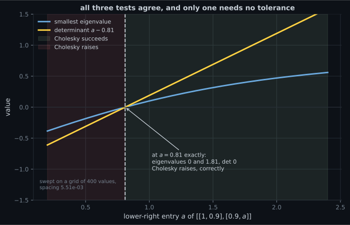
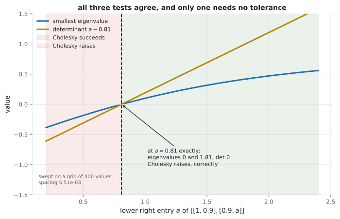
And there is the definiteness test, sitting in the second formula. If $\mathbf{A}$ is not positive definite, the quantity under some square root comes out negative and the algorithm stops. Not “produces a bad answer” — stops, with no tolerance to choose. That is why every numerical library uses Cholesky to test definiteness and why the Inner Products page recommended it over comparing eigenvalues to zero.

What it buys

Solving systems. $\mathbf{A}\mathbf{x} = \mathbf{b}$ becomes $\mathbf{L}(\mathbf{L}^\top\mathbf{x}) = \mathbf{b}$: solve $\mathbf{L}\mathbf{y} = \mathbf{b}$ by forward substitution, then $\mathbf{L}^\top\mathbf{x} = \mathbf{y}$ by back substitution. Two $O(n^2)$ sweeps after one $O(n^3/3)$ factorisation — and if you have many right-hand sides you pay the factorisation once. General LU costs about $2n^3/3$, so Cholesky is a factor of two cheaper, exactly because symmetry means half the matrix is redundant.

Determinants. Since $\det(\mathbf{L}) = \prod_i l_{ii}$ for a triangular matrix (§4.1, Equation 4.8),

$$\det(\mathbf{A}) = \det(\mathbf{L})\det(\mathbf{L}^\top) = \det(\mathbf{L})^2 = \prod_{i=1}^{n} l_{ii}^2$$

The book notes this is why many numerical packages compute determinants this way.

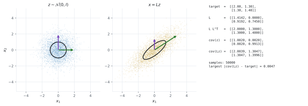
Sampling and the reparametrisation trick. If $\mathbf{z} \sim \mathcal{N}(\mathbf{0}, \mathbf{I})$ then $\mathbf{L}\mathbf{z}$ has covariance

$$\mathrm{Cov}[\mathbf{L}\mathbf{z}] = \mathbf{L}\,\mathrm{Cov}[\mathbf{z}]\,\mathbf{L}^\top = \mathbf{L}\mathbf{I}\mathbf{L}^\top = \mathbf{L}\mathbf{L}^\top = \mathbf{A}$$

So to sample from a Gaussian with a prescribed covariance, factor the covariance and multiply white noise by the factor. The book points forward to §6.5 for the distribution and to the variational autoencoder literature for why this matters: the transformation is a differentiable function of $\mathbf{L}$, so gradients pass through the sampling step. That is the reparametrisation trick.

From the book

Section 4.3. Theorem 4.18 with Equation 4.44 defines the decomposition and asserts uniqueness of the Cholesky factor. Example 4.10 works the $3\times3$ symbolically: Equation 4.45 sets up $\mathbf{A} = \mathbf{L}\mathbf{L}^\top$, Equation 4.46 multiplies out the right-hand side, and Equations 4.47 and 4.48 read off the diagonal and sub-diagonal patterns respectively. The closing paragraph names three uses: manipulating the SPD covariance matrix of a multivariate Gaussian (§6.5), generating samples from that Gaussian, and performing a linear transformation of random variables, which is heavily exploited when computing gradients in deep stochastic models such as the variational autoencoder. It also notes that $\det(\mathbf{A}) = \prod_i l_{ii}^2$ makes determinants efficient and that many numerical software packages use Cholesky for exactly that.

Worked example by hand

Take

$$\mathbf{A} = \begin{bmatrix} 4 & 12 & -16\\ 12 & 37 & -43\\ -16 & -43 & 98\end{bmatrix}$$

Symmetric by inspection. Now run Equations 4.47 and 4.48 in order.

step	formula	working	value
$l_{11}$	$\sqrt{a_{11}}$	$\sqrt{4}$	$2$
$l_{21}$	$a_{21}/l_{11}$	$12/2$	$6$
$l_{31}$	$a_{31}/l_{11}$	$-16/2$	$-8$
$l_{22}$	$\sqrt{a_{22} - l_{21}^2}$	$\sqrt{37 - 36}$	$1$
$l_{32}$	$(a_{32} - l_{31}l_{21})/l_{22}$	$(-43 - (-8)(6))/1 = (-43+48)/1$	$5$
$l_{33}$	$\sqrt{a_{33} - (l_{31}^2 + l_{32}^2)}$	$\sqrt{98 - (64 + 25)} = \sqrt{9}$	$3$

$$\mathbf{L} = \begin{bmatrix} 2 & 0 & 0\\ 6 & 1 & 0\\ -8 & 5 & 3\end{bmatrix}$$

Check by multiplying back. The $(3,3)$ entry: $(-8)^2 + 5^2 + 3^2 = 64 + 25 + 9 = 98$ ✓. The $(3,2)$ entry: $(-8)(6) + (5)(1) = -48 + 5 = -43$ ✓. The $(2,2)$ entry: $6^2 + 1^2 = 37$ ✓.

Every entry of $\mathbf{L}$ is an integer, so $\mathbf{L}\mathbf{L}^\top$ reproduces $\mathbf{A}$ exactly — largest gap $0$, not $10^{-16}$.

The determinant, two ways. From the Cholesky factor:

$$\det\mathbf{A} = (l_{11}l_{22}l_{33})^2 = (2 \cdot 1 \cdot 3)^2 = 36$$

exactly. np.linalg.det, which runs an LU factorisation in floating point, returns $35.999999999999936$. Multiplying the eigenvalues gives $35.99999999999596$ — worse still, because the eigenvalues themselves are computed iteratively. Here the Cholesky route is the most accurate of the three, and it is the cheapest.

Note also that this matrix is not especially well behaved: its eigenvalues are $0.018805$, $15.503963$ and $123.477232$, so $\kappa(\mathbf{A}) = 6566$. The smallest eigenvalue is close to zero and the factorisation still comes out in exact integers, because positive definiteness is a strict inequality and $0.0188 > 0$.

cholesky_worked.py

import numpy as np
 
A = np.array([[4.0, 12.0, -16.0], [12.0, 37.0, -43.0], [-16.0, -43.0, 98.0]])
L = np.linalg.cholesky(A)
 
print("L =")
print(L)
print("L L^T reproduces A exactly:", np.array_equal(L @ L.T, A),
      " largest gap:", f"{float(np.abs(L @ L.T - A).max()):.2e}")
 
print()
print("det from Cholesky:  ", float(np.prod(np.diag(L)) ** 2))
print("det from numpy:     ", float(np.linalg.det(A)))
print("det from eigenvalues:", float(np.prod(np.linalg.eigvalsh(A))))
print("eigenvalues:", np.round(np.linalg.eigvalsh(A), 6),
      " condition number:", round(float(np.linalg.cond(A)), 1))
 
# Solving with L: forward substitution, then back substitution.
def forward(L, b):
    y = np.zeros_like(b)
    for i in range(len(b)):
        y[i] = (b[i] - L[i, :i] @ y[:i]) / L[i, i]
    return y
 
def backward(U, y):
    x = np.zeros_like(y)
    for i in reversed(range(len(y))):
        x[i] = (y[i] - U[i, i + 1:] @ x[i + 1:]) / U[i, i]
    return x
 
rng = np.random.default_rng(5)
b = rng.normal(size=3)
x_chol = backward(L.T, forward(L, b))
x_solve = np.linalg.solve(A, b)
print()
print("x via two triangular solves:", np.round(x_chol, 10))
print("x via np.linalg.solve:      ", np.round(x_solve, 10))
print("gap:", f"{float(np.abs(x_chol - x_solve).max()):.2e}")

output

L =
[[ 2.  0.  0.]
 [ 6.  1.  0.]
 [-8.  5.  3.]]
L L^T reproduces A exactly: True  largest gap: 0.00e+00
 
det from Cholesky:   36.0
det from numpy:      35.999999999999936
det from eigenvalues: 35.99999999999596
eigenvalues: [  0.018805  15.503963 123.477232]  condition number: 6566.2
 
x via two triangular solves: [-22.15612322   6.00547068  -0.98480708]
x via np.linalg.solve:       [-22.15612322   6.00547068  -0.98480708]
gap: 3.91e-14

np.array_equal(L @ L.T, A) returning True is worth pausing on — that is bit-for-bit equality, not approximate agreement, and it happens because every intermediate value in the factorisation is a small integer.

See it move

The first sketch runs Equations 4.47 and 4.48 entry by entry, with the matrix under your control so you can watch the algorithm fail at the moment a square root goes negative.

sketch Cholesky, entry by entry p5.js Pause Restart

Edit the three free entries of a symmetric 3 by 3 and step through the six formulas. Each cell of L lights up as it is computed, with the arithmetic shown. Push the matrix out of positive definiteness and the step that takes a square root of a negative number turns red — which is the definiteness test, happening inside the algorithm.

The second sketch is the sampling application: white noise in, prescribed covariance out.

sketch L turns white noise into correlated samples p5.js Pause Restart

Drag the three entries of the target covariance. The left cloud is standard normal noise, the right is that noise multiplied by the Cholesky factor, and the ellipse on each is the one-sigma contour of the measured sample covariance. The readout compares the measured covariance against the target you asked for.

From scratch

cholesky_from_scratch.py

import numpy as np
 
def cholesky(A, tol=0.0):
    """Equations 4.47 and 4.48, in general form. Raises on non-SPD input."""
    A = np.asarray(A, dtype=float)
    n = A.shape[0]
    if not np.allclose(A, A.T):
        raise ValueError("not symmetric")
    L = np.zeros((n, n))
    for i in range(n):
        for j in range(i + 1):
            s = float(A[i, j] - L[i, :j] @ L[j, :j])
            if i == j:
                if s <= tol:
                    raise ValueError(f"not positive definite: "
                                     f"sqrt of {s:.6g} at position ({i}, {i})")
                L[i, i] = np.sqrt(s)
            else:
                L[i, j] = s / L[j, j]
    return L
 
A = np.array([[4.0, 12.0, -16.0], [12.0, 37.0, -43.0], [-16.0, -43.0, 98.0]])
L = cholesky(A)
print("our L:"); print(L)
print("numpy agrees:", np.allclose(L, np.linalg.cholesky(A)))
print("uniqueness — every entry identical:", np.array_equal(L, np.linalg.cholesky(A)))
 
# It is also the definiteness test, with no tolerance to pick.
print()
for a in (0.85, 0.81, 0.80):
    M = np.array([[1.0, 0.9], [0.9, a]])
    try:
        cholesky(M)
        verdict = "positive definite"
    except ValueError as e:
        verdict = str(e)
    print(f"a = {a}:  det {float(np.linalg.det(M)):+.6f}  "
          f"smallest eigenvalue {float(np.linalg.eigvalsh(M)[0]):+.8f}  ->  {verdict}")
 
# The log determinant, which never overflows.
print()
rng = np.random.default_rng(23)
for n in (10, 100, 150, 175):
    M = rng.normal(size=(n, n))
    S = M @ M.T + n * np.eye(n)
    Ln = np.linalg.cholesky(S)
    det = float(np.linalg.det(S))
    logdet = 2.0 * float(np.sum(np.log(np.diag(Ln))))
    print(f"n = {n:4}:  det {det:12.4e}  finite {str(np.isfinite(det) and det > 0):5}  "
          f"2*sum(log diag L) = {logdet:.4f}")

output

our L:
[[ 2.  0.  0.]
 [ 6.  1.  0.]
 [-8.  5.  3.]]
numpy agrees: True
uniqueness — every entry identical: True
 
a = 0.85:  det +0.040000  smallest eigenvalue +0.02188041  ->  positive definite
a = 0.81:  det +0.000000  smallest eigenvalue +0.00000000  ->  not positive definite: sqrt of 0 at position (1, 1)
a = 0.8:  det -0.010000  smallest eigenvalue -0.00553851  ->  not positive definite: sqrt of -0.01 at position (1, 1)
 
n =   10:  det   8.1875e+12  finite True   2*sum(log diag L) = 29.7336
n =  100:  det  1.8120e+225  finite True   2*sum(log diag L) = 518.6761
n =  150:  det          inf  finite False  2*sum(log diag L) = 837.9401
n =  175:  det          inf  finite False  2*sum(log diag L) = 1005.9729

Three results. The from-scratch factor is bit-for-bit identical to numpy’s, which is what “unique” means made concrete. The boundary case $a = 0.81$ fails with sqrt of 0 — a determinant of exactly zero and a smallest eigenvalue of exactly zero, and the algorithm rejects it without being asked to compare anything against a tolerance. And by $n = 150$ the determinant has overflowed to inf while the log determinant is a perfectly ordinary $837.94$.

On real data

figure White noise in, prescribed covariance out matplotlib

Fifty thousand samples. L L-transpose reproduces the target exactly, and the measured covariance of Lz differs from the target by at most 0.0047 — sampling error, not a modelling gap. The two arrows are the unit vectors, pushed through L.

figure Three definiteness tests, one boundary matplotlib

At a = 0.81 the matrix is positive semidefinite: eigenvalues 0 and 1.81, determinant 0. Cholesky raises there, correctly — the strict inequality of Definition 3.2 is the one it enforces, and it needs no tolerance to do so.

figure Why the log determinant is what libraries store matplotlib

On the right the direct determinant overflows to inf at n = 150 while 2 times the sum of the log diagonal keeps rising smoothly past n = 175. Every Gaussian log-likelihood in Chapter 6 is written in the second form for this reason.

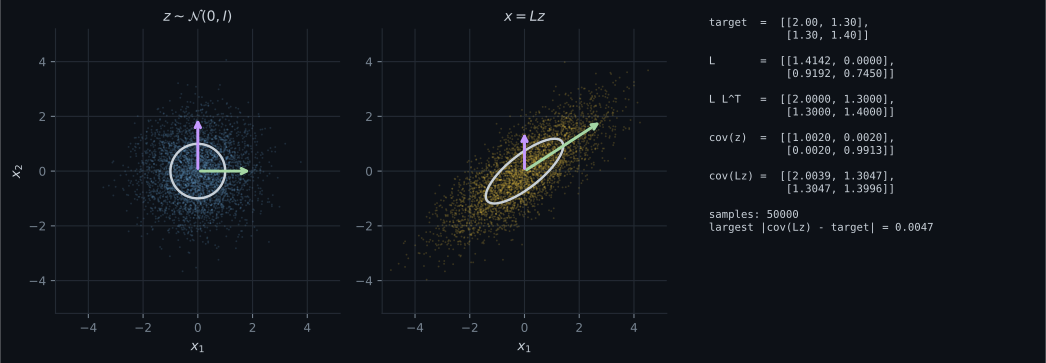
Reading the plot

From the sampling figure. The identity being verified is $\mathrm{Cov}[\mathbf{L}\mathbf{z}] = \mathbf{L}\mathbf{L}^\top$, and the check has two halves. The algebraic half is exact: $\mathbf{L}\mathbf{L}^\top$ reproduces the target to the printed precision. The empirical half is not, and should not be: the measured covariance of $50{,}000$ samples differs from the target by at most $0.0047$, which is sampling error.

That distinction matters when debugging. If the measured covariance is off, first check whether the gap shrinks as $1/\sqrt{n}$: measured here at $0.39$ for $100$ samples, $0.12$ for $1000$, $0.0096$ for $10{,}000$ and $0.0047$ for $50{,}000$ — a factor of about $3$ per factor of $10$, which is $\sqrt{10} \approx 3.16$. If it does not shrink that way, the bug is in the transformation, not the sample size.

From the boundary figure. The three tests agree on where positive definiteness ends, and they differ in what they need from you. The determinant crossing zero and the smallest eigenvalue crossing zero are both continuous quantities you must compare against a threshold. Cholesky is a branch: the square root either has a positive argument or it does not.

At $a = 0.81$ exactly, the matrix has eigenvalues $0$ and $1.81$ — positive semidefinite. Definition 3.2 asks for the strict inequality, so the right answer is to reject it, and Cholesky does. A test written as all(eigvalsh(A) >= 0) would accept it, which is the failure mode the Inner Products page measured.

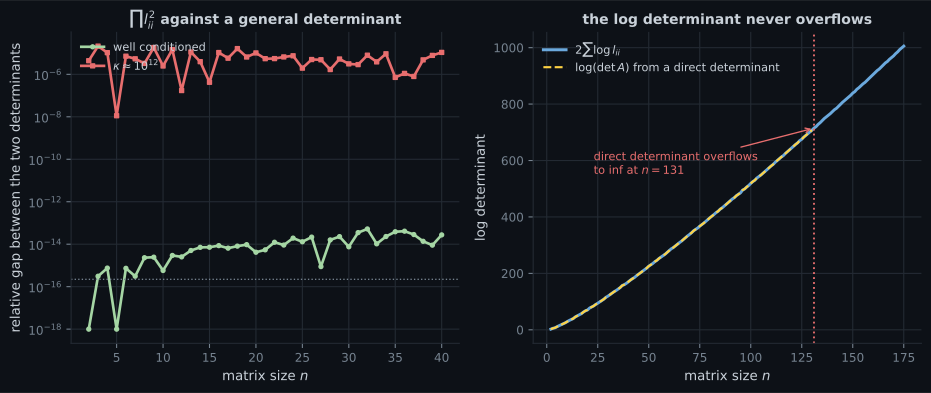
From the determinant figure. The right panel is the practical one. The direct determinant is finite up to about $n = 120$ and inf from about $n = 150$; the log determinant is $837.94$ there and keeps going. Nothing has gone wrong with the matrix — a $150\times150$ SPD matrix with entries of order $10$ simply has a determinant around $e^{838} \approx 10^{364}$ — past the largest double, whose exponent stops near $10^{308}$.

The left panel is the accuracy story, and it is more subtle. On well-conditioned input both routes agree to machine precision. On input with $\kappa \approx 10^{12}$ they diverge — and note which direction the argument runs: the worked $3\times3$ on this page has $\kappa = 6566$ and the Cholesky determinant is exactly $36$ while numpy’s general determinant gives $35.999999999999936$. Cholesky is more accurate there because it exploits symmetry and does half the arithmetic. But it is not universally more accurate; for a nearly-singular matrix the square roots amplify error too, which is what the ill conditioned curve shows.

Pitfalls

Cholesky is not a general “matrix square root”

It requires symmetric and positive definite. Not symmetric positive semidefinite — a covariance matrix estimated from fewer samples than dimensions is singular and Cholesky will refuse it. Not symmetric indefinite. Not non-symmetric at all. If you need a factor for a semidefinite matrix, use an eigendecomposition with the negative-but-tiny eigenvalues clipped to zero, and say in your code that you did.

Adding jitter changes the answer, so report the jitter

The standard fix for a nearly-singular covariance is $\mathbf{A} + \varepsilon\mathbf{I}$, which is what makes the factorisation succeed. It also changes every downstream number: the samples you draw have covariance $\mathbf{A} + \varepsilon\mathbf{I}$, not $\mathbf{A}$, and the log determinant is inflated by roughly $n\varepsilon / \bar{\lambda}$. The book mentions the same “jitter term” for the pseudo-inverse in §3.8.2 and notes it can be derived as a ridge prior. It is a modelling decision wearing numerical clothing.

np.linalg.cholesky returns lower triangular; scipy defaults to upper

np.linalg.cholesky(A) gives $\mathbf{L}$ with $\mathbf{A} = \mathbf{L}\mathbf{L}^\top$. scipy.linalg.cholesky(A) gives $\mathbf{U}$ with $\mathbf{A} = \mathbf{U}^\top\mathbf{U}$ unless you pass lower=True. Mixing the two silently transposes your factor, which produces the right covariance and the wrong correlation structure — a bug that passes a covariance check and fails a sample check.

Do not compute the determinant when you want the log determinant

np.log(np.linalg.det(A)) overflows to inf and then to nan for moderate $n$, and loses precision long before that. Use $2\sum_i \log l_{ii}$ from the Cholesky factor. It is cheaper, it never overflows, and it is already what you need for a Gaussian log-likelihood.

Symmetry has to be exact enough

np.linalg.cholesky reads only the lower triangle, so it will happily factor a matrix that is not symmetric, using half of it and ignoring the rest. If your matrix should be symmetric and is not — a covariance built as X.T @ X / n picks up asymmetry of order $10^{-16}$, which is fine, but one built by hand may not — symmetrise explicitly with (A + A.T) / 2 before factoring, and check the size of what you discarded.

Compare

decomposition	needs	gives	cost	unique?
Cholesky $\mathbf{L}\mathbf{L}^\top$	symmetric positive definite	a triangular square root	$n^3/3$	yes
LU	square, invertible (with pivoting)	two triangular factors	$2n^3/3$	up to pivoting
QR	any	orthonormal $\times$ triangular	$2mn^2$	up to column signs
eigendecomposition	square, non-defective	eigenbasis $\times$ diagonal	$\approx 10n^3$	no: signs, ordering
SVD	any	rotation $\times$ scale $\times$ rotation	$\approx 20n^3$	up to paired signs

Cholesky is the cheapest and the most restrictive, which is the usual trade. When your matrix qualifies — and covariance matrices, kernel matrices and Hessians at a minimum routinely do — it is the right tool.

pch.quizTag Check your understanding

1. Why does Theorem 4.18 require A to be symmetric, separately from requiring positive definiteness?

   A It does not; positive definiteness implies symmetry B Because L L-transpose is symmetric for any L whatsoever, so a non-symmetric A cannot be written in that form at all — while positive definiteness is what keeps the square roots real C To make the factorisation unique D To make the determinant positive
   pch.quizShowAnswer

   B — Because L L-transpose is symmetric for any L whatsoever, so a non-symmetric A cannot be written in that form at all — while positive definiteness is what keeps the square roots real — The two hypotheses do different jobs. Symmetry makes the shape possible; positive definiteness makes the arithmetic possible, because Equation 4.47 takes square roots of quantities that positive definiteness keeps positive.

2. The from-scratch Cholesky of the worked 3x3 is bit-for-bit identical to numpy's. What does that illustrate?

   A That numpy uses the same code B Uniqueness: Theorem 4.18 says the Cholesky factor of a given SPD matrix is one specific matrix, so any correct implementation must return it — unlike an eigendecomposition, where signs and orderings are free C That the matrix is diagonal D That floating point is exact
   pch.quizShowAnswer

   B — Uniqueness: Theorem 4.18 says the Cholesky factor of a given SPD matrix is one specific matrix, so any correct implementation must return it — unlike an eigendecomposition, where signs and orderings are free — Bit-for-bit agreement here also depends on every intermediate value being a small integer. On generic input the agreement would be to machine precision rather than exact, but the factor would still be mathematically unique.

3. At a = 0.81 the matrix [[1, 0.9], [0.9, a]] has eigenvalues 0 and 1.81. Cholesky raises. Is that right?

   A No, it should succeed since no eigenvalue is negative B Yes. The matrix is positive SEMIdefinite and Definition 3.2 asks for the strict inequality, so it must be rejected — and Cholesky rejects it without needing any tolerance, where a test written as all eigenvalues at least zero would wrongly accept it C It depends on the tolerance D Only for 2x2 matrices
   pch.quizShowAnswer

   B — Yes. The matrix is positive SEMIdefinite and Definition 3.2 asks for the strict inequality, so it must be rejected — and Cholesky rejects it without needing any tolerance, where a test written as all eigenvalues at least zero would wrongly accept it — The error message is 'sqrt of 0', which is the algorithm's own report of the boundary. That branch-not-threshold behaviour is the whole reason to prefer Cholesky as a definiteness test.

4. For a 150x150 SPD matrix, np.linalg.det returns inf while 2 times the sum of the log diagonal of L returns 838.93. What should you conclude?

   A The matrix is singular B Nothing is wrong with the matrix — its determinant is genuinely around e to the 838, which is about 10 to the 364 and past the largest double at 10 to the 308, so the quantity to compute is the log determinant rather than the determinant C The Cholesky factorisation failed D The matrix is badly conditioned
   pch.quizShowAnswer

   B — Nothing is wrong with the matrix — its determinant is genuinely around e to the 838, which is about 10 to the 364 and past the largest double at 10 to the 308, so the quantity to compute is the log determinant rather than the determinant — Its condition number is fine. This is why every Gaussian log-likelihood is written with a log determinant term computed from a Cholesky factor rather than by taking the log of a determinant.

5. In the sampling figure the measured covariance differs from the target by 0.0047 at 50000 samples. How do you tell whether that is a bug?

   A Any nonzero gap is a bug B Check whether it shrinks like one over the square root of the sample count — measured 0.39 at 100 samples, 0.12 at 1000, 0.0096 at 10000, 0.0047 at 50000, which is roughly a factor of 3 per factor of 10 in n C Compare against the determinant D Increase the jitter
   pch.quizShowAnswer

   B — Check whether it shrinks like one over the square root of the sample count — measured 0.39 at 100 samples, 0.12 at 1000, 0.0096 at 10000, 0.0047 at 50000, which is roughly a factor of 3 per factor of 10 in n — The algebraic identity Cov[Lz] = L L-transpose is exact; what remains is sampling error. If the gap does not shrink at that rate, the transformation is wrong — a transposed factor being the classic cause.

🧪 Try It Yourself

Exercise 1 – Cholesky by hand

pch.exerciseTag pch.exerciseTitle

Exercise 2 – The general algorithm

pch.exerciseTag pch.exerciseTitle

Exercise 3 – Cholesky as the definiteness test

pch.exerciseTag pch.exerciseTitle

Exercise 4 – Solve a system with the factor

pch.exerciseTag pch.exerciseTitle

Exercise 5 – The log determinant does not overflow

pch.exerciseTag pch.exerciseTitle

Recall card

• Cholesky factors a symmetric positive definite matrix as L L-transpose, with L lower triangular and positive on the diagonal, and L is unique — unlike an eigendecomposition, where signs and orderings are free.
• Symmetry makes the shape possible and positive definiteness makes the arithmetic possible: L L-transpose is symmetric for any L, and positive definiteness is what keeps every square root real.
• The entries come out one at a time, each from entries of A and entries of L already known, in a single sweep with no iteration.
• The factorisation is the definiteness test. It stops when a square root would go negative, so it needs no tolerance — and at the semidefinite boundary it correctly rejects a matrix that “all eigenvalues at least zero” would accept.
• The determinant is the squared product of the diagonal, which is cheaper than a general determinant and, on the worked example, more accurate: exactly 36 against numpy’s 35.999999999999936.
• Use the log determinant, twice the sum of the logs of the diagonal. A direct determinant overflows to infinity by about n = 150 on a perfectly well-conditioned matrix.
• L z has covariance L L-transpose when z is standard normal, which is how you sample a Gaussian with a prescribed covariance — and because the map is differentiable in L, it is the reparametrisation trick.
• It costs half of an LU factorisation, n cubed over three against two n cubed over three, because symmetry makes half the matrix redundant.
• Adding jitter to make it succeed changes the model, not just the arithmetic. Report the epsilon.

Next: Eigendecomposition and Diagonalization — the factorisation that uses §4.2’s eigenvectors as its basis.