
Useful Identities for Computing Gradients
§5.5 is a page of the book and a table of ten equations. It states them, cites Petersen and Pedersen’s Matrix Cookbook, and proves none of them.
That is a reasonable choice for a textbook and a bad situation for a reader, because a memorised identity you cannot check is worse than no identity at all — you will use it, get a plausible number, and not find out. So this page does two things: verifies all ten against independent finite differences, and isolates the two places where the stated form differs from the shortcut people actually write, with the size of the error when they do.
Both of those are about symmetry, and both are off by tens of percent.
What you’ll learn
Section titled “What you’ll learn”- All ten identities, Equations 5.99 to 5.108, each verified numerically.
- Why Equation 5.107 says and not — with the 29% error the shortcut costs.
- Why Equation 5.108 carries the clause “for symmetric ” — with the 107% error when it is not.
- Which identities are the same statement in different clothes, and which are genuinely independent.
- The cost question the section raises without answering: if a library differentiates anything, why memorise these? Measured.
- The book’s own caveat about traces and transposes of higher-order tensors.
Intuition: the identities are differentials
Section titled “Intuition: the identities are differentials”Every line in §5.5 is a differential — a statement about what happens to the output when you nudge the input — rather than a four-index tensor. That is why they are usable, and it is the whole reason the section exists directly after §5.4’s tensors.
Read as: nudge , and the inverse moves by minus the inverse, times the nudge in , times the inverse again. No index ever appears. Contracting §5.4’s tensor against a direction gives exactly this, which the previous page measured.
  flowchart TD
  T["§5.4: the derivative is a
fourth-order tensor"]
  T -->|"contract with a direction"| D["a DIFFERENTIAL:
a statement about one nudge"]
  D --> L["§5.5's ten identities
Eq 5.99 – 5.108"]
  L --> STRUCT["structural, about any f:
5.99 transpose · 5.100 trace
5.101 determinant · 5.102 inverse"]
  L --> CONC["concrete, for specific forms:
5.103 aᵀX⁻¹b · 5.104/5.105 aᵀx
5.106 aᵀXb · 5.107 xᵀBx · 5.108 least squares"]
  CONC --> TRAP1["5.107: (B + Bᵀ), not 2B
the shortcut is 29% wrong"]
  CONC --> TRAP2["5.108: 'for symmetric W'
without it, 107% wrong"]
  TRAP1 --> WHY["both traps are the same fact:
a quadratic form only sees
the symmetric part of its matrix"]
  TRAP2 --> WHY
  L --> CAVEAT["the book's Remark: trace and
transpose are not defined for
higher-order tensors — that is
a tensor contraction"]
The math
Section titled “The math”The ten identities
Section titled “The ten identities”That remark is doing real work. Equations 5.99 to 5.102 are written with and applied to , which for a matrix argument is a tensor — so those symbols mean contractions, not the matrix operations they look like. In practice you apply the identity in a direction, where everything is a matrix again.
Which of these are actually different statements
Section titled “Which of these are actually different statements”Ten equations, fewer ideas.
| identities | what they really are |
|---|---|
| 5.104, 5.105 | the same identity. because an inner product is symmetric, so there is one fact here, listed twice for lookup convenience |
| 5.106 | 5.104 with a matrix in the middle. Setting to basis vectors picks out a single entry |
| 5.103 | 5.106 composed with 5.102: differentiate , then sandwich |
| 5.107 | the only genuinely quadratic one, and the only one where symmetry appears explicitly |
| 5.108 | 5.107 composed with the chain rule and a linear inner function — and it is Chapter 9’s gradient |
| 5.99–5.102 | structural: true for any differentiable , not for a specific form |
So the list is four structural rules and three independent concrete ones, with the rest following by composition. Worth knowing, because it tells you which ones to memorise: 5.102 and 5.107, and 5.108 because you will use it constantly.
The two traps
Section titled “The two traps”Both are the same fact wearing different hats: a quadratic form only ever sees the symmetric part of its matrix.
For any , write with symmetric and antisymmetric. Then
because is its own negative transpose. So , and differentiating gives — Equation 5.107.
Trap one. Writing instead is right precisely when is symmetric. Measured on a random :
| form | relative error against a finite difference |
|---|---|
120% wrong — the error is larger than the gradient itself. And with a symmetric
the two forms agree to 0.0e+00, so the bug is invisible on every
symmetric test case you might try first.
Trap two. Equation 5.108’s clause “for symmetric ” is not decoration. The general result is
and the factor of appears only when . Measured:
| Equation 5.108 as stated | the general form | |
|---|---|---|
| symmetric | ||
| not symmetric |
Read the first two rows across: for a symmetric the stated form and the general form give the same number, because exactly. No symmetric test can tell them apart. On the third row the stated form is wrong while the general form stays at .
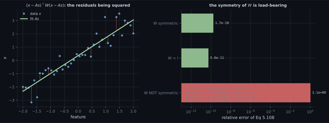
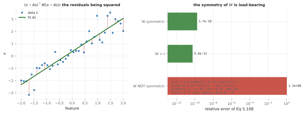
(The figure below uses a different matrix and gets — — for the same failure. How wrong the shortcut is depends on how far from symmetric is; that it is wrong does not.)
In practice is usually symmetric — it is an inverse covariance, or the identity — which is exactly why the clause gets forgotten.
Worked example by hand
Section titled “Worked example by hand”Equation 5.107, derived twice
Section titled “Equation 5.107, derived twice”By coordinates. . Differentiate with respect to : the variable appears once as the index and once as the index, so the product rule gives two terms,
and collecting into a row gives . The two terms are where the transpose comes from — one for each occurrence of .
By differential. Nudge by :
The two first-order terms are scalars, so each equals its own transpose: . Adding them,
Two lines, no indices. This is the method to use.
Equation 5.108, from 5.107 and the chain rule
Section titled “Equation 5.108, from 5.107 and the chain rule”Let and . Then by §5.3’s chain rule,
using Equation 5.107 for the first factor and Example 5.9 for the second. If this collapses to , which is Equation 5.108. And with it is Example 5.11’s — the same identity, three times, at increasing generality.
Equation 5.102, and why the minus sign
Section titled “Equation 5.102, and why the minus sign”From , differentiate both sides. The right side is constant, so
which is Equation 5.102. The minus sign is not a convention — it comes from moving a term across an equals sign, and the two factors come from multiplying through on both sides. In one dimension this is , which is the same statement with the order irrelevant.
All ten, checked
Section titled “All ten, checked”import numpy as np
def numeric_jac(f, x, h=1e-6):
"""Central-difference Jacobian of a flattened function of a flat input."""
x = np.asarray(x, dtype=float).ravel()
f0 = np.asarray(f(x)).ravel()
J = np.zeros((f0.size, x.size))
for j in range(x.size):
e = np.zeros_like(x)
e[j] = h
J[:, j] = (np.asarray(f(x + e)).ravel() - np.asarray(f(x - e)).ravel()) / (2 * h)
return J
rng = np.random.default_rng(19)
n, h = 3, 1e-6
fX = lambda M: M @ M # any smooth matrix function
tests = []
# 5.99 d f(X)^T = (d f(X))^T, in a direction H
X, H = rng.normal(size=(n, n)), rng.normal(size=(n, n))
tests.append(("5.99", (fX(X + h*H).T - fX(X - h*H).T) / (2*h),
((fX(X + h*H) - fX(X - h*H)) / (2*h)).T))
# 5.100 d tr(f) = tr(d f)
tests.append(("5.100", np.array([[(np.trace(fX(X + h*H)) - np.trace(fX(X - h*H))) / (2*h)]]),
np.array([[np.trace((fX(X + h*H) - fX(X - h*H)) / (2*h))]])))
# 5.101 d det(f) = det(f) tr(f^-1 d f)
Xp, Hp = rng.normal(size=(n, n)) + 3*np.eye(n), rng.normal(size=(n, n))
dfp = (fX(Xp + h*Hp) - fX(Xp - h*Hp)) / (2*h)
tests.append(("5.101",
np.array([[(np.linalg.det(fX(Xp + h*Hp)) - np.linalg.det(fX(Xp - h*Hp))) / (2*h)]]),
np.array([[np.linalg.det(fX(Xp)) * np.trace(np.linalg.inv(fX(Xp)) @ dfp)]])))
# 5.102 d f^-1 = -f^-1 (d f) f^-1
tests.append(("5.102", (np.linalg.inv(fX(Xp + h*Hp)) - np.linalg.inv(fX(Xp - h*Hp))) / (2*h),
-np.linalg.inv(fX(Xp)) @ dfp @ np.linalg.inv(fX(Xp))))
# 5.103 d(a^T X^-1 b)/dX = -(X^-1)^T a b^T (X^-1)^T
Xi = rng.normal(size=(n, n)) + 3*np.eye(n)
a, b = rng.normal(size=n), rng.normal(size=n)
Xinv = np.linalg.inv(Xi)
tests.append(("5.103", numeric_jac(lambda v: np.array([a @ np.linalg.inv(v.reshape(n, n)) @ b]), Xi),
(-Xinv.T @ np.outer(a, b) @ Xinv.T).reshape(1, -1)))
# 5.104 and 5.105 d(x^T a)/dx = a^T = d(a^T x)/dx
x, av = rng.normal(size=n), rng.normal(size=n)
tests.append(("5.104", numeric_jac(lambda v: np.array([v @ av]), x), av.reshape(1, -1)))
tests.append(("5.105", numeric_jac(lambda v: np.array([av @ v]), x), av.reshape(1, -1)))
# 5.106 d(a^T X b)/dX = a b^T
Xm = rng.normal(size=(n, n))
tests.append(("5.106", numeric_jac(lambda v: np.array([a @ v.reshape(n, n) @ b]), Xm),
np.outer(a, b).reshape(1, -1)))
# 5.107 d(x^T B x)/dx = x^T (B + B^T)
B = rng.normal(size=(n, n))
tests.append(("5.107", numeric_jac(lambda v: np.array([v @ B @ v]), x),
(x @ (B + B.T)).reshape(1, -1)))
# 5.108 d/ds (x - As)^T W (x - As) = -2 (x - As)^T W A, W symmetric
m = 4
Aw = rng.normal(size=(m, n))
W0 = rng.normal(size=(m, m)); W = W0 + W0.T
xw, s0 = rng.normal(size=m), rng.normal(size=n)
r = xw - Aw @ s0
tests.append(("5.108", numeric_jac(lambda v: np.array([(xw - Aw @ v) @ W @ (xw - Aw @ v)]), s0),
(-2 * r @ W @ Aw).reshape(1, -1)))
errs = []
for name, num, ana in tests:
num = np.asarray(num, float)
ana = np.asarray(ana, float).reshape(num.shape)
e = float(np.abs(num - ana).max()) / max(float(np.abs(ana).max()), 1e-12)
errs.append(e)
print(f" {name:>7} relative error {e:.2e}")
print(f" worst of the ten: {max(errs):.1e}") 5.99 relative error 0.00e+00
5.100 relative error 2.51e-11
5.101 relative error 1.29e-10
5.102 relative error 4.71e-11
5.103 relative error 2.71e-10
5.104 relative error 4.00e-11
5.105 relative error 4.00e-11
5.106 relative error 5.25e-11
5.107 relative error 8.70e-11
5.108 relative error 1.46e-10
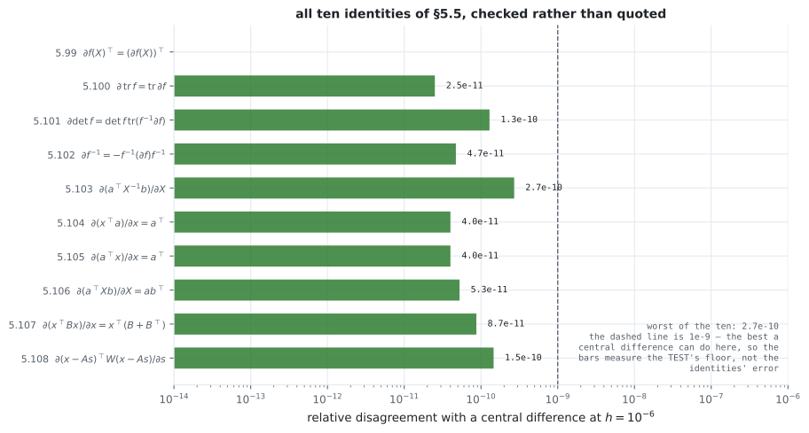
worst of the ten: 2.7e-10Two readings.
Equation 5.99’s error is exactly 0.00e+00. That is not machine precision, it is
identically zero — the two sides are the same four numbers rearranged, because
transposing before or after a difference of transposes is the same set of
subtractions. A check that comes out exactly zero is checking the algebra rather
than the analysis.
The other nine are between and , which is the test’s floor rather than the identities’. §5.1’s figure showed a central difference at cannot do better than about relative. So these say “consistent with exact”, and the two traps below sit at and — nine orders away.
See it move
Section titled “See it move”From scratch
Section titled “From scratch”import numpy as np
def numeric_jac(f, x, h=1e-6):
x = np.asarray(x, dtype=float).ravel()
f0 = np.asarray(f(x)).ravel()
J = np.zeros((f0.size, x.size))
for j in range(x.size):
e = np.zeros_like(x)
e[j] = h
J[:, j] = (np.asarray(f(x + e)).ravel() - np.asarray(f(x - e)).ravel()) / (2 * h)
return J
rng = np.random.default_rng(31)
# ---- Trap one: Eq 5.107 is (B + B^T), not 2B.
print("Trap one: d(x^T B x)/dx")
B = rng.normal(size=(4, 4))
x = rng.normal(size=4)
num = numeric_jac(lambda v: np.array([v @ B @ v]), x)
right = (x @ (B + B.T)).reshape(1, -1)
wrong = (2 * x @ B).reshape(1, -1)
scale = float(np.abs(right).max())
print(f" x^T(B + B^T) relative error {float(np.abs(num - right).max()) / scale:.2e}")
print(f" 2 x^T B relative error {float(np.abs(num - wrong).max()) / scale:.2e}")
Bs = B + B.T # now symmetric
num2 = numeric_jac(lambda v: np.array([v @ Bs @ v]), x)
r2 = (x @ (Bs + Bs.T)).reshape(1, -1)
w2 = (2 * x @ Bs).reshape(1, -1)
print(f" with a SYMMETRIC B the two forms differ by {float(np.abs(r2 - w2).max()):.1e}")
print(f" -- so the shortcut passes every symmetric test case")
# And why: the antisymmetric part contributes nothing to the form itself.
Ba = (B - B.T) / 2
vals = [float(v @ Ba @ v) for v in rng.normal(size=(5, 4))]
print(f" x^T B_a x for five random x: {[f'{v:.1e}' for v in vals]}")
# ---- Trap two: Eq 5.108 needs W symmetric.
print()
print("Trap two: d/ds (x - As)^T W (x - As)")
m, d = 6, 3
A = rng.normal(size=(m, d))
xv = rng.normal(size=m)
s0 = rng.normal(size=d)
e0 = xv - A @ s0
for label, W in (("symmetric", (lambda M: M + M.T)(rng.normal(size=(m, m)))),
("identity", np.eye(m)),
("NOT symmetric", rng.normal(size=(m, m)))):
num = numeric_jac(lambda v: np.array([(xv - A @ v) @ W @ (xv - A @ v)]), s0)
stated = (-2 * e0 @ W @ A).reshape(1, -1) # Eq 5.108 as written
general = (-e0 @ (W + W.T) @ A).reshape(1, -1) # the general form
sc = max(float(np.abs(num).max()), 1e-12)
print(f" W {label:14} Eq 5.108 as stated {float(np.abs(num - stated).max())/sc:9.2e}"
f" general form {float(np.abs(num - general).max())/sc:9.2e}")Trap one: d(x^T B x)/dx
x^T(B + B^T) relative error 8.78e-11
2 x^T B relative error 1.20e+00
with a SYMMETRIC B the two forms differ by 0.0e+00
-- so the shortcut passes every symmetric test case
x^T B_a x for five random x: ['3.5e-18', '-4.2e-16', '3.5e-18', '-5.4e-17', '-1.4e-16']
Trap two: d/ds (x - As)^T W (x - As)
W symmetric Eq 5.108 as stated 1.26e-10 general form 1.26e-10
W identity Eq 5.108 as stated 8.70e-11 general form 8.70e-11
W NOT symmetric Eq 5.108 as stated 2.86e-01 general form 6.57e-12The two rows to read are the last two.
For a symmetric the stated identity and the general form give the same answer — because exactly. So there is no test with a symmetric that can distinguish them, and inverse covariances are symmetric, and the identity matrix is symmetric.
For a non-symmetric the stated identity is off by while the general form stays at — four orders apart on the same input. The clause “for symmetric ” is the whole difference.
And the last line of the first block explains both traps: comes out between and for five random — zero to within rounding. The antisymmetric part is invisible to the form, so it cannot appear in the derivative, so any expression that retains it is wrong by exactly the amount it retains.
On real data
Section titled “On real data”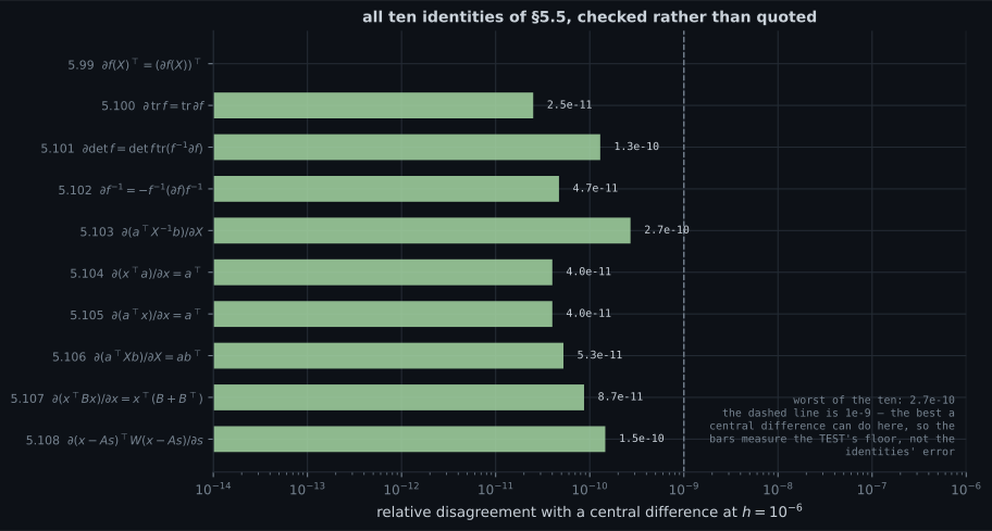
Reading the plot
Section titled “Reading the plot”From the ten-identities figure. The bars span to , and the useful thing about that narrow range is that it is uninformative about the identities: it is the resolution of the test. What would be informative is a bar at , and the next figure has one.
Two bars are worth naming. Equation 5.99 at exactly 0.0e+00 — the algebra, not the
analysis, as discussed above. And Equation 5.103 at , the worst of
the ten, which is expected: it differentiates through a matrix inverse, and inverting
a amplifies input perturbations by its condition number, so the difference
quotient has further to fall before it converges.
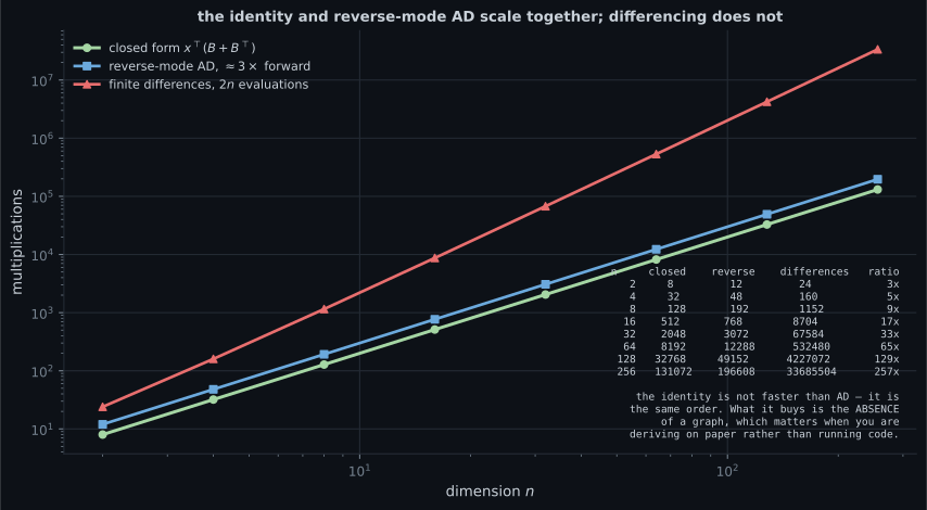
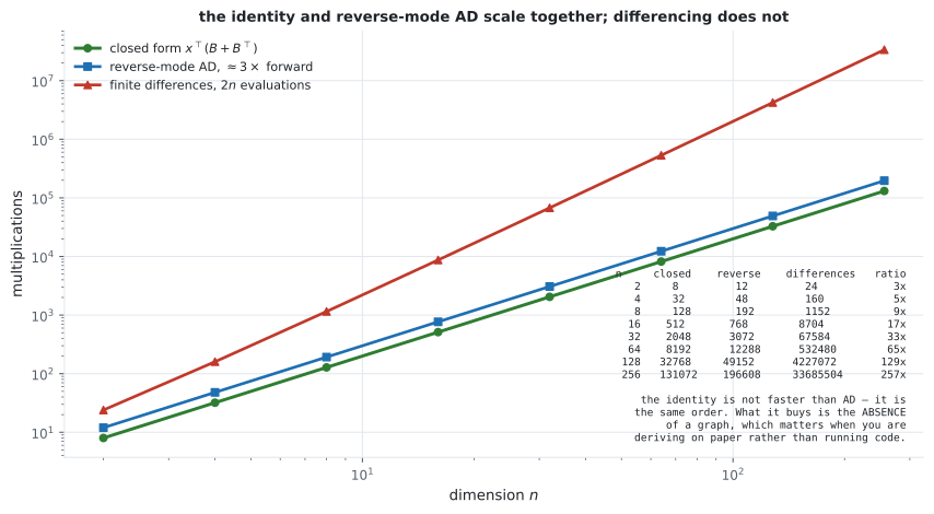
From the cost figure. The green and blue lines being parallel is the answer to the question the section raises. A closed-form identity is multiplications and reverse-mode autodiff is about — the same order, a constant factor apart. So memorising identities does not buy asymptotic speed over a library.
What it buys is visible in the red line and in the ratio:
| closed form | reverse AD | differencing | ratio | |
|---|---|---|---|---|
The ratio is exactly , which falls straight out of the arithmetic: . So differencing is not a constant factor worse, it is a factor of the dimension worse — which is the real reason nobody gradient-checks a large model except on a tiny slice.
And the honest summary of the identities: they are for deriving on paper. When you are writing code, use the library; when you are working out what the gradient is, these ten lines are what you have.
From the symmetry figure. The right panel is the only bar chart in this module with a bar at : for a symmetric , for the identity, and — — for a non-symmetric one. The failing case is the one you would never test, because is almost always symmetric.
The left panel is there to say what the objective is: those vertical red segments
are the residuals, and decides how much each one counts. With
they count equally, which is ordinary least squares; with
they are weighted by certainty, which is
Chapter 9’s generalised least squares. Both symmetric. The clause survives because
the case that violates it does not arise — until someone writes
W = np.random.randn(m, m) in a test.
Pitfalls
Section titled “Pitfalls”Compare
Section titled “Compare”| identity | the shortest way to see it | where it is used |
|---|---|---|
| 5.99 transpose | both sides are the same entries reindexed | rearranging derivations |
| 5.100 trace | the trace is a sum, and differentiation is linear | Ch 6 Gaussian log-densities |
| 5.101 determinant | Jacobi’s formula; from and 5.102 | Ch 6 change of variables, normalising flows |
| 5.102 inverse | differentiate and move a term | Ch 9 posterior updates |
| 5.103 | 5.106 composed with 5.102 | Gaussian conditionals |
| 5.104 = 5.105 | an inner product is symmetric | everywhere |
| 5.106 | 5.104 with a matrix inserted | picking out matrix entries |
| 5.107 quadratic | two terms because appears twice | every quadratic loss, every Hessian |
| 5.108 least squares | 5.107 then the chain rule then Example 5.9 | Ch 9’s starting point |
The three in bold are the ones to memorise. The rest you can rebuild from them in a line or two, which is a better use of memory than a lookup table you cannot check.
-
Why does Equation 5.107 say x-transpose times (B plus B-transpose) rather than 2 x-transpose B?
Measured on a random 4x4: the shortcut is off by 1.20 relative — 120 percent, a larger error than the gradient is large. And for symmetric B the two forms agree to exactly 0.0e+00, so the shortcut passes every symmetric test case you would think to write.
pch.quizShowAnswer
B — Because differentiating the double sum hits x_k twice — once as the row index and once as the column index — giving Bx plus B-transpose x. Writing 2B keeps the antisymmetric part, which the quadratic form cannot see — Measured on a random 4x4: the shortcut is off by 1.20 relative — 120 percent, a larger error than the gradient is large. And for symmetric B the two forms agree to exactly 0.0e+00, so the shortcut passes every symmetric test case you would think to write.
-
Both traps on this page come from the same underlying fact. What is it?
Measured: x-transpose B_a x came out between 3.5e-18 and 4.2e-16 for five random x — zero to within rounding. Any expression for the gradient that retains B_a — like 2 x-transpose B, or Eq 5.108 with a non-symmetric W — is wrong by exactly that retained part.
pch.quizShowAnswer
B — That a quadratic form only sees the symmetric part of its matrix: x-transpose times the antisymmetric part times x is exactly zero for every x, so that part cannot appear in the derivative — Measured: x-transpose B_a x came out between 3.5e-18 and 4.2e-16 for five random x — zero to within rounding. Any expression for the gradient that retains B_a — like 2 x-transpose B, or Eq 5.108 with a non-symmetric W — is wrong by exactly that retained part.
-
The ten identity bars all sit between 2.5e-11 and 2.7e-10. What does that range tell you?
A test whose resolution is 1e-10 can only ever say 'consistent with exact'. The value of the check is that a wrong form lands nine orders away: the two traps on this page measure 1.20 and 2.9e-01.
pch.quizShowAnswer
B — Almost nothing about the identities — it is the central difference's own floor at h = 1e-6. What would be informative is a bar at 1e-1, and the symmetry figure has one at 1.07 — A test whose resolution is 1e-10 can only ever say 'consistent with exact'. The value of the check is that a wrong form lands nine orders away: the two traps on this page measure 1.20 and 2.9e-01.
-
The cost figure shows finite differencing costing exactly n+1 times the closed form. Where does that come from?
So differencing is not a constant factor worse, it is a factor of the DIMENSION worse: 3x at n = 2 and 257x at n = 256. That is why nobody gradient-checks a large model except on a tiny slice.
pch.quizShowAnswer
B — From the arithmetic: differencing needs 2n evaluations of a form costing n-squared plus n, over a closed form costing 2 n-squared — which simplifies to n+1 exactly — So differencing is not a constant factor worse, it is a factor of the DIMENSION worse: 3x at n = 2 and 257x at n = 256. That is why nobody gradient-checks a large model except on a tiny slice.
-
Given that a closed form and reverse-mode autodiff are the same order, what are these ten identities actually for?
2n-squared against 3n-squared is a constant factor, so hand-derived gradients buy no asymptotic speed and cost a maintenance burden whenever the model changes. The measured lines are parallel on the log-log plot, which is the whole point.
pch.quizShowAnswer
B — Deriving on paper. They need no computation graph, so they are what you use to work out what a gradient IS, and to sanity-check a library on a small case — not to replace the library — 2n-squared against 3n-squared is a constant factor, so hand-derived gradients buy no asymptotic speed and cost a maintenance burden whenever the model changes. The measured lines are parallel on the log-log plot, which is the whole point.
🧪 Try It Yourself
Section titled “🧪 Try It Yourself”Exercise 1 – All ten identities
Section titled “Exercise 1 – All ten identities”Exercise 2 – Trap one: why (B + B-transpose)
Section titled “Exercise 2 – Trap one: why (B + B-transpose)”Exercise 3 – Trap two: Equation 5.108’s symmetry clause
Section titled “Exercise 3 – Trap two: Equation 5.108’s symmetry clause”Exercise 4 – The cost of each route
Section titled “Exercise 4 – The cost of each route”Exercise 5 – Rebuild 5.103 and 5.108 by composition
Section titled “Exercise 5 – Rebuild 5.103 and 5.108 by composition”Recall card
Section titled “Recall card”- Every identity in §5.5 is a differential — a statement about one nudge — which is why they are usable by hand where §5.4’s tensors are not.
- Ten equations, fewer ideas. 5.99 to 5.102 are structural rules for any f; 5.104 and 5.105 are the same fact; 5.103 is 5.106 composed with 5.102; 5.108 is 5.107 plus the chain rule. Memorise 5.102, 5.107 and 5.108.
- All ten verified against central differences: worst relative error 2.7e-10, which is the test’s floor rather than the identities’.
- Equation 5.99 comes out at exactly 0.0e+00, because both sides are the same numbers rearranged — a check on the algebra, not the analysis.
- Trap one: Equation 5.107 is x-transpose (B + B-transpose), not 2 x-transpose B. The shortcut is off by 1.20 relative on a general B — more than the gradient itself — and exactly right on a symmetric one, so it passes every symmetric test case.
- Trap two: Equation 5.108’s ‘for symmetric W’ is load-bearing. With a non-symmetric W the stated form is off by 2.9e-01 in one test and 1.07 in another, while the general form — minus e-transpose (W + W-transpose) A — stays at 1e-12.
- Both traps are the same fact: a quadratic form only sees the symmetric part of its matrix, because x-transpose times the antisymmetric part times x is zero for every x — measured between 3.5e-18 and 4.2e-16.
- The trace and transpose in 5.99 to 5.102 mean contractions when f takes a matrix argument — the book’s own Remark says the matrix operations are undefined for higher-order tensors.
- Differencing costs exactly n+1 times a closed form — 3x at n = 2, 257x at n = 256 — because it needs 2n evaluations of an n-squared form.
- A closed form and reverse-mode AD are the same order, 2n² against 3n². Identities buy understanding and paper derivations, not speed.
Next: Backpropagation and Automatic Differentiation — the chain rule applied mechanically, and why it costs about what the function costs.
pch.coffeeTagline
pch.coffeeCtapch.feedbackHeading
pch.feedbackSubheading