Chapter 12 Worked Problems

These are not the book’s exercises

Chapter 12 of Mathematics for Machine Learning has no end-of-chapter exercises — it runs from §12.1 to §12.6 and then into the references. Every problem below is this module’s own, built from claims the chapter makes, with the relevant section named. Nothing here should be attributed to Deisenroth, Faisal and Ong.

#	problem	sections	the answer in one line
1	Does a large margin really generalise?	§12.2.1	reliably good, reliably not optimal — the $84$th percentile
2	What does a change of units cost?	§12.2.1	$0.2638$ of held-out accuracy, on data that never moved
3	What does the support vector count tell you?	§12.3.1	a leave-one-out bound, tight when separated and loose when not
4	How do you choose $C$?	§12.2.4	cross-validation; and the plateau is wide
5	How do $C$ and $\gamma$ interact?	§12.4	not independently — a small $\gamma$ needs a large $C$
6	Will the SVM give you a probability?	§12.6	no; $74\%$ of its scores fall outside $[-1, 1]$
7	SVM against logistic regression	§12.6	one has support vectors because its loss reaches zero
8	What does class imbalance do?	§12.2.4	recall on the minority collapses to $0.0000$ while accuracy looks fine

All eight use the tools of pages 1201–1209, plus scikit-learn’s SVC — which wraps LIBSVM, one of the two implementations §12.5 names.

Problem 1 — Does a large margin really generalise?

Statement. The book asserts it in a margin note: “A classifier with large margin turns out to generalize well.” Page 1201 measured a correlation of $0.590999$ on one dataset. One dataset is one draw.

Method. Generate $200$ separable training sets of $10$ points each, fit the hard-margin SVM, and compare its held-out accuracy against thousands of other hyperplanes that also separate the same training data perfectly.

text

  datasets compared                        : 192
  SVM beats every sampled separator        : 6
  SVM at or above the median               : 184
  SVM below the median                     : 8
  mean percentile of the SVM among them    : 84.11%
  mean gap to the BEST sampled separator   : -0.00819
  worst gap to the best sampled separator  : -0.18250

Answer. The max-margin rule is reliably good and reliably not optimal. It lands at the $84$th percentile on average and beats every sampled alternative on only $6$ of $192$ datasets. On average it gives up $0.00819$ of accuracy against the best separator that existed — and on the worst dataset, $0.18250$.

That is not a criticism. Nothing computable from the training set could have identified the better separator; it was better by luck. What the margin buys is the $84$th percentile every time, which is exactly what page 1201’s binned table showed from the other direction: the worst case per margin bin rose from $0.8757$ to $0.9777$ while the best barely moved.

Problem 2 — What does a change of units cost?

Statement. Page 1202 found that an anisotropic rescale moves the classifier, but could not show it on the running example, whose separator is already axis-aligned. Build a case where it bites.

Method. Note first what rescaling actually does. Fitting on $\mathbf{S}\mathbf{x}$ with $\mathbf{S} = \mathrm{diag}(1, s)$ and mapping back is equivalent to minimising

$$w_1^2 + \frac{w_2^2}{s^2}$$

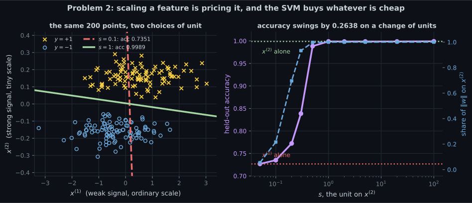
under the original constraints. So $s$ is a price on using feature 2. Build data where the cheap feature is the bad one: $x^{(1)}$ weakly informative on an ordinary scale, $x^{(2)}$ strongly informative on a tiny one.

problem_2.py

import numpy as np
from sklearn.svm import SVC
 
SIG1, SD1 = 0.60, 1.00        # weak signal, ordinary scale
SIG2, SD2 = 0.15, 0.05        # strong signal, tiny scale
 
rg = np.random.default_rng(4)
def make(m):
    y = np.r_[np.ones(m // 2), -np.ones(m // 2)]
    return np.c_[rg.normal(SIG1 * y, SD1), rg.normal(SIG2 * y, SD2)], y
 
XA, YA = make(200)
XT, YT = make(20000)
print(f"threshold on x1 alone : "
      f"{float((np.where(XT[:, 0] >= 0, 1.0, -1.0) == YT).mean()):.4f}")
print(f"threshold on x2 alone : "
      f"{float((np.where(XT[:, 1] >= 0, 1.0, -1.0) == YT).mean()):.4f}")
 
print(f"{'s on x2':>9} {'w (orig coords, unit)':>25} {'|w2| share':>11} "
      f"{'held-out acc':>13}")
for s in (0.1, 0.5, 1.0, 2.0, 5.0, 20.0, 100.0):
    m = SVC(C=1.0, kernel="linear", tol=1e-8).fit(XA * np.array([1.0, s]), YA)
    w = np.array([m.coef_[0, 0], m.coef_[0, 1] * s])
    b = float(m.intercept_[0])
    un = w / np.linalg.norm(w)
    acc = float((np.where(XT @ w + b >= 0, 1.0, -1.0) == YT).mean())
    print(f"{s:>9.1f} {str(np.round(un, 6)):>25} {abs(un[1]):>11.4f} "
          f"{acc:>13.4f}")

text

threshold on x1 alone : 0.7267
threshold on x2 alone : 0.9989
  s on x2     w (orig coords, unit)  |w2| share  held-out acc
      0.1       [0.976353 0.216181]      0.2162        0.7351
      0.5       [0.067737 0.997703]      0.9977        0.9884
      1.0       [0.022453 0.999748]      0.9997        0.9989
      2.0       [0.020694 0.999786]      0.9998        0.9987
      5.0       [0.023274 0.999729]      0.9997        0.9988
     20.0       [0.013963 0.999903]      0.9999        0.9988
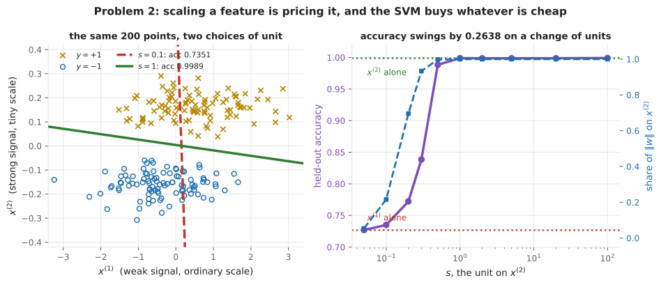
    100.0       [0.005857 0.999983]      1.0000        0.9991

Answer. Held-out accuracy swings by $0.2638$ on a change of units. At $s = 0.1$ the fitted weight is $97.6\%$ on $x^{(1)}$ and the classifier scores $0.7351$ — essentially the $x^{(1)}$-only figure of $0.7267$. At $s = 1$ it is $99.97\%$ on $x^{(2)}$ and scores $0.9989$, exactly the $x^{(2)}$-only figure.

The regulariser $\tfrac12\lVert\mathbf{w}\rVert^2$ treats every coordinate of $\mathbf{w}$ alike, so a feature measured in small units needs a large weight and is therefore expensive. The SVM buys whatever is cheap, and the units decide what is cheap.

Standardising both features first removes the choice:

$s$	held-out accuracy, standardised
$0.1$	$0.9962$
$1.0$	$0.9989$
$100.0$	$0.9991$

The spread collapses from $0.2638$ to $0.0029$. This is §10.6’s standardisation decision appearing in Chapter 12, with nothing said about it anywhere in the chapter.

figure Problem 2: scaling a feature is pricing it, and the SVM buys whatever is cheap matplotlib

The classes are cleanly separated top from bottom, and at s = 0.1 the SVM draws a vertical line anyway — because using the vertical coordinate would cost twenty times more weight. The blue dashed curve on the right is the share of ||w|| the fit puts on that coordinate.

Problem 3 — What does the support vector count tell you?

Statement. Page 1206 measured that deleting a non-support vector leaves the solution unchanged. That has a consequence the chapter never draws: it bounds the leave-one-out error.

Reasoning. Delete example $n$ and refit. If $n$ was not a support vector the solution is identical, so the refit still classifies $n$ correctly. Every leave-one-out mistake must therefore come from a support vector, giving

$$\text{LOO error} \;\leq\; \frac{\#\{n : \alpha_n > 0\}}{N}$$

Method. Fit once to count support vectors, then run all $N$ leave-one-out refits and compare.

text

                   dataset     N   #SV    bound  true LOO  bound holds
            well separated    60     2   0.0333    0.0000         True
               overlapping    60    12   0.2000    0.0833         True
             heavy overlap    60    33   0.5500    0.2333         True
     well separated, N=120   120     2   0.0167    0.0167         True

Answer. The bound holds everywhere, and it is useful exactly when the data is separable. On well-separated data two support vectors bound the leave-one-out error at $0.0333$ — a real guarantee from a single fit. Under heavy overlap $33$ of $60$ examples are support vectors and the bound reads $0.5500$ against a true $0.2333$: true, and worth nothing.

The reason is page 1206’s box constraint. When the data overlaps, most support vectors sit at $\alpha_n = C$ rather than strictly inside, and deleting one of those changes the solution very little — so the bound counts them as potential errors when they are not.

Problem 4 — How do you choose C?

Statement. §12.2.4 introduces $C$ and never says how to set it. Page 1204 mapped what it does; this is how to pick it.

text

         C   train acc   5-fold CV   held-out    #SV
     0.001      0.8400      0.8400     0.8516    200
     0.010      0.8750      0.8700     0.8636    132
     0.100      0.8750      0.8750     0.8683     81
     1.000      0.8750      0.8800     0.8682     64
    10.000      0.8750      0.8800     0.8689     62
   100.000      0.8750      0.8800     0.8689     62
  1000.000      0.8750      0.8800     0.8689     62

Answer. Cross-validation picks $C = 1$, and the plateau is four orders of magnitude wide. Everything from $C = 0.1$ to $C = 1000$ scores between $0.8682$ and $0.8689$ held out, against a Bayes rate of $0.8682$ for this generator.

Three things worth reading off:

• Training accuracy is useless here. It is $0.8750$ for every $C$ above $0.001$ and cannot distinguish a model that stores $200$ support vectors from one that stores $62$.
• The support vector count keeps falling after accuracy stops improving, from $200$ to $62$. If two settings score the same, the one with fewer support vectors is cheaper to evaluate.
• The SVM matches the Bayes rate, and at $C \geq 10$ exceeds it by $0.0007$. On a finite test set that is luck, not superiority — page 1109 measured the same effect for the GMM classifier.

Problem 5 — How do C and gamma interact?

Statement. §12.4 says the kernel’s parameters “are often chosen using nested cross-validation” but does not say whether they can be chosen one at a time.

text

   gamma      C=0.1       C=1      C=10     C=100    C=1000
    0.01     0.7143    0.7210    0.9942    0.9958    0.9965
    0.10     0.9940    0.9955    0.9952    0.9935    0.9815
    1.00     0.9912    0.9950    0.9918    0.9898    0.9898
   10.00     0.9210    0.9898    0.9905    0.9905    0.9905
  100.00     0.7530    0.8287    0.8375    0.8375    0.8375

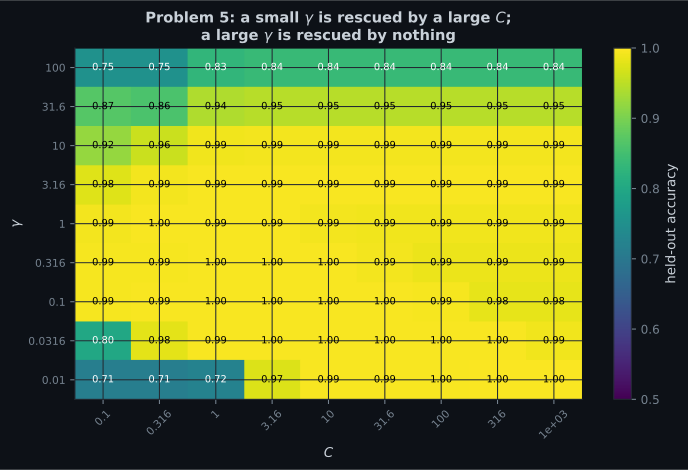
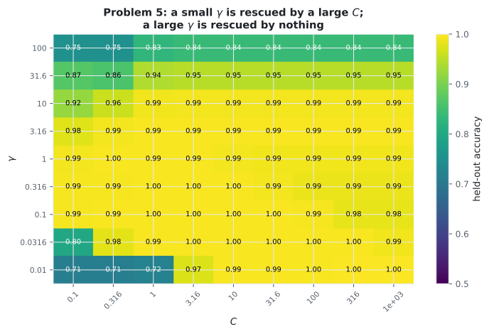
Answer. They cannot. Read the $\gamma = 0.01$ row: $0.7143$ at $C = 0.1$ and $0.9965$ at $C = 1000$. A kernel too wide to separate the rings is rescued entirely by making violations expensive enough. Now read $\gamma = 100$: $0.7530$ to $0.8375$, and no value of $C$ rescues it — the kernel is so narrow that every point is its own island.

So the interaction is one-sided. A small $\gamma$ can be compensated by a large $C$; a large $\gamma$ cannot be compensated by anything. Tuning $\gamma$ first at a fixed $C = 1$ would have picked $\gamma = 0.1$ and missed that $\gamma = 0.01$ with $C = 1000$ is better.

figure Problem 5: a small gamma is rescued by a large C; a large gamma is rescued by nothing matplotlib

The bottom row is the interaction: 0.71 at C = 0.1 and 1.00 at C = 1000, same kernel. The top rows are the asymmetry: no column helps. This is why the two are searched on a grid rather than in sequence.

Problem 6 — Will the SVM give you a probability?

Statement. §12.6 is explicit: “The SVM is a binary classifier that does not naturally lend itself to a probabilistic interpretation.” It names Platt scaling as the repair. How good is it?

text

  decision values range over [-7.907, 8.012]
  fraction outside [-1, 1]  : 0.7440
 
                             model   accuracy     Brier   log loss
               SVM + Platt scaling     0.8696   0.09695    0.31606
               logistic regression     0.8694   0.09540    0.30715
                the true posterior     0.8682   0.09538    0.30703

Answer. The raw decision values are not probabilities and are not close to being any — they span $[-7.907, 8.012]$ and $74.40\%$ of them fall outside $[-1, 1]$ altogether. Squashing them needs the extra calibration step the section describes.

The three-row comparison is the useful part. The data here was generated from two Gaussians with equal covariance, for which the true posterior is a logistic function of $\mathbf{x}$ — so logistic regression has the correct model class and lands essentially on the truth ($0.09540$ against $0.09538$). Platt-scaled SVM scores $0.09695$, worse on both proper scoring rules while being marginally more accurate ($0.8696$ against $0.8694$).

That is the trade in one table: the SVM optimises the decision boundary, and pays for it in the probabilities.

Problem 7 — SVM against logistic regression

Statement. §12.6 names logistic regression as the maximum-likelihood counterpart. Their losses differ in exactly one structural respect.

$t = y f(\mathbf{x})$	hinge	logistic $\log(1+e^{-t})$
$-2.0$	$3.0000$	$2.126928$
$0.0$	$1.0000$	$0.693147$
$1.0$	$\mathbf{0.0000}$	$0.313262$
$2.0$	$\mathbf{0.0000}$	$0.126928$
$5.0$	$\mathbf{0.0000}$	$0.006715$
$10.0$	$\mathbf{0.0000}$	$0.000045$

The hinge reaches exactly zero; the logistic loss never does. Delete the five examples the SVM ignores on the running example and refit both:

text

  the SVM's support vectors : [0, 1, 4]  (3 of 8)
 
      SVM, C = 1e4 : angle after deleting the other 5 =  0.000000 deg, offset moves 0.000000
   logistic, C = 1 : angle after deleting the other 5 =  0.000000 deg, offset moves 0.537167

Answer. The SVM is bit-for-bit unchanged; logistic regression’s offset moves by $0.537167$. The direction happened to be preserved for both, because this dataset is symmetric — but the SVM’s invariance is structural and logistic regression’s is an accident of the example.

That is the whole difference. A loss that reaches zero produces support vectors; a loss that only approaches zero keeps every example in the solution forever. Page 1205 measured the same property from the primal side, and page 1206 from the dual side as $\alpha_n = 0$.

Problem 8 — What does class imbalance do?

Statement. Nothing in Chapter 12 mentions class balance. Equation 12.26a charges $C$ per unit of slack regardless of which class produced it.

text

 positives  negatives   accuracy  recall on +  always -1 acc
       100        200     0.8003       0.6775         0.5000
        50        200     0.7360       0.5115         0.5000
        20        200     0.6100       0.2230         0.5000
        10        200     0.5000       0.0000         0.5000
         5        200     0.5000       0.0000         0.5000

Answer. At ten positives against two hundred negatives the SVM predicts $-1$ for everything. Recall on the positive class is exactly $0.0000$, and the model is useless — but its accuracy on a balanced held-out set is still $0.5000$, which does not look like total failure. On an imbalanced held-out set it would read $0.9524$ and look excellent.

The cause is Equation 12.26a. Misclassifying all ten positives costs $10C$ of slack; buying them back requires moving the boundary into two hundred negatives. The objective is doing exactly what it was asked to do, and what it was asked is not what anyone wanted.

The standard repair is a per-class $C$ — $C_+ = C\cdot N/(2N_+)$ and $C_- = C\cdot N/(2N_-)$ — which is a change to the problem, not to the solver, and belongs to the same family as page 1204’s remark about which terms carry a coefficient.

pch.quizTag Check your understanding

1. A The margin principle is wrong B The sampling was inadequate C Maximising the margin is reliably good and reliably not optimal — nothing computable from the training set could have found the better separators, which were better by luck D A larger training set would make it optimal
   pch.quizShowAnswer

   C — Maximising the margin is reliably good and reliably not optimal — nothing computable from the training set could have found the better separators, which were better by luck

2. A Because it changes the labels B Because fitting on the scaled data is equivalent to minimising w1 squared plus w2 squared over s squared under the original constraints — so s is a price on using that feature C Because the data becomes non-separable D Because the kernel changes
   pch.quizShowAnswer

   B — Because fitting on the scaled data is equivalent to minimising w1 squared plus w2 squared over s squared under the original constraints — so s is a price on using that feature

3. A Always; it is tight by construction B When the data is well separated — 2 support vectors of 60 gives a bound of 0.0333 from one fit. Under heavy overlap 33 of 60 are support vectors and the bound reads 0.5500 against a true 0.2333 C Only for non-separable data D Never; it does not hold
   pch.quizShowAnswer

   B — When the data is well separated — 2 support vectors of 60 gives a bound of 0.0333 from one fit. Under heavy overlap 33 of 60 are support vectors and the bound reads 0.5500 against a true 0.2333

4. A That gamma should always be small B That C should always be large C That the two parameters interact asymmetrically: a small gamma can be compensated by a large C, but a large gamma cannot be compensated by anything — so they must be searched jointly D That the RBF kernel is unsuitable here
   pch.quizShowAnswer

   C — That the two parameters interact asymmetrically: a small gamma can be compensated by a large C, but a large gamma cannot be compensated by anything — so they must be searched jointly

5. A Yes; the optimisation failed to converge B No — Equation 12.26a charges C per unit of slack regardless of class, so misclassifying all ten positives is cheaper than moving the boundary into two hundred negatives. The objective is doing what it was asked C Yes; the data is not separable D No, but only because C was too large
   pch.quizShowAnswer

   B — No — Equation 12.26a charges C per unit of slack regardless of class, so misclassifying all ten positives is cheaper than moving the boundary into two hundred negatives. The objective is doing what it was asked

Exercises

Exercise 1 – Price a feature by rescaling it

pch.exerciseTag pch.exerciseTitle

Exercise 2 – Bound the leave-one-out error from one fit

pch.exerciseTag pch.exerciseTitle

Exercise 3 – Show the two knobs are not independent

pch.exerciseTag pch.exerciseTitle

Exercise 4 – Show that the SVM does not produce probabilities

pch.exerciseTag pch.exerciseTitle

Exercise 5 – Watch imbalance eat the minority class

pch.exerciseTag pch.exerciseTitle

Recall card

• A large margin is reliably good and reliably not optimal. Across 192 separable datasets the max-margin solution averaged the 84th percentile among separators that fit the training data equally well, and beat all of them only 6 times.
• It gives up 0.00819 of accuracy on average against the best separator that existed, and 0.18250 on the worst dataset — but nothing computable from the training set could have found those.
• Scaling a feature is pricing it. Fitting on scaled data is the same as minimising a weighted norm under the original constraints, so the unit you choose decides how expensive each feature is to use.
• Measured, that is worth 0.2638 of held-out accuracy — the SVM puts 97.6 percent of its weight on the weak feature when the strong one is made expensive. Standardising first collapses the spread to 0.0029.
• The support vector count bounds the leave-one-out error, because deleting a non-support vector cannot change the solution.
• That bound is worth having only when the data separates. Two support vectors of sixty give a guarantee of 0.0333; thirty-three of sixty give 0.5500 against a true 0.2333.
• C’s good plateau is four orders of magnitude wide on ordinary data, and training accuracy cannot see any of it — but the support vector count keeps falling long after accuracy stops rising.
• C and gamma interact asymmetrically. A kernel too wide is rescued entirely by a large C, from 0.7143 to 0.9965; a kernel too narrow is rescued by nothing, staying below 0.8375 for every C.
• So tuning them in sequence misses the best cell, which is why Section 12.4 refers to nested cross-validation over both.
• The SVM’s raw output is not a probability and is not close to one. Nearly three quarters of its scores fall outside the unit interval.
• Platt scaling repairs that at a cost. Against a generator whose true posterior is logistic, logistic regression essentially matches the truth on both proper scores while the calibrated SVM does not — and the SVM is marginally more accurate.
• The hinge reaches exactly zero and the logistic loss never does, which is the entire reason one has support vectors and the other does not. Deleting the ignored examples leaves the SVM bit-for-bit identical and moves logistic regression’s offset by 0.537167.
• Class imbalance is invisible to accuracy and fatal to the minority class. At ten positives against two hundred negatives the recall on positives is exactly zero while balanced accuracy still reads 0.5000.

Next: Chapter 12 Formula Sheet — every equation, every measured constant, on one page.