Numerical Solution

Everything so far has been a derivation. Section 12.5 asks the practical question: given all these equivalent formulations, which one do you hand to a solver, and what does it cost?

The hinge has one kink, and Equation 12.54 covers it

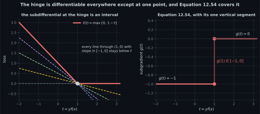
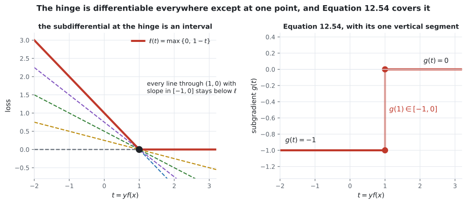
Equation 12.31 is convex and unconstrained, so gradient descent is the obvious method — except the hinge is not differentiable at $t = 1$. The fix is a subgradient:

$$g(t) = \begin{cases} -1 & t < 1\\ [-1, 0] & t = 1\\ 0 & t > 1 \end{cases} \qquad \text{(12.54)}$$

A number $g$ is a subgradient of $\ell$ at $t_0$ when $\ell(t) \geq \ell(t_0) + g\,(t - t_0)$ for every $t$ — geometrically, when the line through $(t_0, \ell(t_0))$ with slope $g$ stays below the loss everywhere. At the kink a whole interval of slopes qualifies:

which_slopes_qualify.py

import numpy as np
 
ts = np.linspace(-6, 6, 240001)
lt = np.maximum(0.0, 1 - ts)                 # the hinge loss
 
print(f"{'candidate g':>13} {'valid at t0 = 1?':>18} {'worst violation':>17}")
for g in (-1.5, -1.0, -0.7, -0.5, -0.25, 0.0, 0.25):
    viol = float(np.max(0.0 + g * (ts - 1.0) - lt))   # l(t0) = 0 at t0 = 1
    print(f"{g:>13.2f} {str(viol <= 1e-12):>18} {max(viol, 0.0):>17.3e}")

text

  candidate g   valid at t0 = 1?   worst violation
        -1.50              False         3.500e+00
        -1.00               True         0.000e+00
        -0.70               True         0.000e+00
        -0.50               True         0.000e+00
        -0.25               True         0.000e+00
         0.00               True         0.000e+00
         0.25              False         1.250e+00

Everything in $[-1, 0]$ qualifies and nothing outside it does. Away from the kink the subgradient is unique — scanning $3{,}001$ candidate slopes at $t_0 = -2$, $0.5$, $2$ and $3$ leaves exactly one valid in each case. That is why Equation 12.54 gives a set at one point and a number everywhere else.

figure The hinge is differentiable everywhere except at one point, and Equation 12.54 covers it matplotlib

The fan of dashed lines is the subdifferential. Any one of them is a legitimate step direction — which is exactly why subgradient descent is slower than gradient descent: the direction is only guaranteed not to point uphill.

What a subgradient costs

subgradient_descent.py

def subgrad(XX, YY, C, iters, eta0=0.5, seed=0):
    d = XX.shape[1]
    rg = np.random.default_rng(seed)
    w, b = rg.normal(0, 0.3, d), float(rg.normal(0, 0.3))
    best = obj(w, b, XX, YY, C)
    for k in range(1, iters + 1):
        t = YY * (XX @ w + b)
        act = t < 1.0                       # 12.54: g = -1 exactly here
        gw = w - C * (YY[act] @ XX[act]) if act.any() else w.copy()
        gb = -C * YY[act].sum() if act.any() else 0.0
        eta = eta0 / k
        w, b = w - eta * gw, b - eta * gb
        best = min(best, obj(w, b, XX, YY, C))   # note: BEST, not last
    return best

text

  iterations    best objective   gap to the QP
          10      3.9235861529       4.859e-02
         100      3.8882244562       1.322e-02
        1000      3.8791122429       4.112e-03
       10000      3.8762946193       1.295e-03
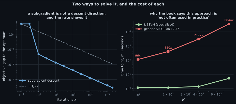
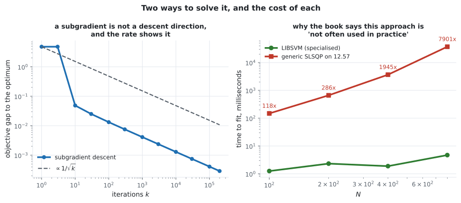
      100000      3.8754091186       4.091e-04

A hundred thousand iterations to reach four decimal places. Each factor of ten in iterations buys roughly a factor of three in accuracy — the $O(1/\sqrt{k})$ rate that is characteristic of subgradient methods, against the linear or quadratic convergence a smooth problem would allow.

Note the best rather than the last iterate. A subgradient step can increase the objective, so the running minimum is what converges; tracking only the current point gives a sequence that wobbles.

Both formulations as standard-form quadratic programs

The book writes each SVM in the standard form of §7.3.2, $\min \tfrac12\mathbf{v}^\top\mathbf{P}\mathbf{v} + \mathbf{q}^\top\mathbf{v}$ subject to $\mathbf{G}\mathbf{v} \leq \mathbf{h}$.

The primal, with variables $[\mathbf{w}; b; \boldsymbol\xi] \in \mathbb{R}^{D+1+N}$:

$$\min_{\mathbf{w}, b, \boldsymbol\xi}\ \frac12 \begin{bmatrix}\mathbf{w}\\ b\\ \boldsymbol\xi\end{bmatrix}^\top \begin{bmatrix}\mathbf{I}_D & \mathbf{0}\\ \mathbf{0} & \mathbf{0}\end{bmatrix} \begin{bmatrix}\mathbf{w}\\ b\\ \boldsymbol\xi\end{bmatrix} + \begin{bmatrix}\mathbf{0}_{D+1}\\ C\mathbf{1}_N\end{bmatrix}^\top \begin{bmatrix}\mathbf{w}\\ b\\ \boldsymbol\xi\end{bmatrix} \quad\text{s.t.}\quad \begin{bmatrix}-\mathbf{Y}\mathbf{X} & -\mathbf{y} & -\mathbf{I}_N\\ \mathbf{0} & \mathbf{0} & -\mathbf{I}_N\end{bmatrix} \begin{bmatrix}\mathbf{w}\\ b\\ \boldsymbol\xi\end{bmatrix} \leq \begin{bmatrix}-\mathbf{1}_N\\ \mathbf{0}_N\end{bmatrix} \qquad \text{(12.55), (12.56)}$$

The dual, with variables $\boldsymbol\alpha \in \mathbb{R}^N$:

$$\min_{\boldsymbol\alpha}\ \tfrac12\boldsymbol\alpha^\top\mathbf{Y}\mathbf{K}\mathbf{Y}\boldsymbol\alpha - \mathbf{1}^\top\boldsymbol\alpha \quad\text{s.t.}\quad \begin{bmatrix}\mathbf{y}^\top\\ -\mathbf{y}^\top\\ -\mathbf{I}_N\\ \mathbf{I}_N\end{bmatrix} \boldsymbol\alpha \leq \begin{bmatrix}\mathbf{0}_2\\ \mathbf{0}_N\\ C\mathbf{1}_N\end{bmatrix} \qquad \text{(12.57)}$$

Both built and solved on the nine-point example, against the reference optimum $3.8750000000$:

form	variables	constraint rows	solved value	gap
primal, 12.56	$D + 1 + N = 12$	$2N = 18$	$3.8750000000$	$7.105\times10^{-15}$
dual, 12.57	$N = 9$	$2N + 2 = 20$	$-3.8750000000$	$2.132\times10^{-14}$

Equation 12.58 is a workaround, and it doubles a row

The dual has the equality $\mathbf{y}^\top\boldsymbol\alpha = 0$, and the standard form only accepts inequalities. Equation 12.58’s fix is to write each equality twice:

$$\mathbf{A}\mathbf{x} = \mathbf{b} \quad\text{becomes}\quad \mathbf{A}\mathbf{x} \leq \mathbf{b} \ \text{ and } \ \mathbf{A}\mathbf{x} \geq \mathbf{b} \qquad \text{(12.58)}$$

That is why the dual’s constraint matrix above has $2N + 2$ rows rather than $2N + 1$: the first two rows are $\mathbf{y}^\top$ and $-\mathbf{y}^\top$, the same constraint from both sides. The book adds that “particular software implementations of convex optimization methods may provide the ability to express equality constraints” — and the ones worth using all do.

Which formulation is smaller?

The primal’s size grows with $D$, the dual’s does not:

setting	$D$	$N$	primal variables	dual variables
the running example	$2$	$9$	$12$	$9$
digits, $8$ vs $3$	$64$	$360$	$425$	$360$
MNIST, two classes	$784$	$12{,}000$	$12{,}785$	$12{,}000$
text, bag of words	$50{,}000$	$2{,}000$	$52{,}001$	$\mathbf{2{,}000}$
genomics	$20{,}000$	$200$	$20{,}201$	$\mathbf{200}$
with an RBF kernel	$\infty$	$1{,}000$	infinite	$\mathbf{1{,}000}$

The last row is the one that matters. An RBF kernel’s feature space has no finite dimension, so the primal has no finite variable count at all — the dual is not merely smaller there, it is the only one of the two that exists. That is the practical payoff of page 1206’s derivation, and page 1208’s rank measurement is the same fact seen from another angle.

“Not often used in practice”

The section ends with an admission:

The approach presented here, expressing the SVM problem in standard convex optimization form, is not often used in practice.

It is worth knowing how large “not often” is. Timing the generic SLSQP solve of Equation 12.57 against LIBSVM — the solver the book cites as one of the two main implementations — on the same data:

text

  N =   200 : LIBSVM       2.8 ms, generic SLSQP      249.3 ms, ratio     89.2x
  N =   800 : LIBSVM       2.4 ms, generic SLSQP    29415.5 ms, ratio  12349.1x
  N =  2000 : LIBSVM      10.2 ms, generic SLSQP   504152.8 ms, ratio  49548.2x

Eight minutes against ten milliseconds at $N = 2000$, and the gap widens with every doubling. The generic solver treats $\mathbf{Y}\mathbf{K}\mathbf{Y}$ as an arbitrary dense quadratic form and maintains an approximation to its inverse; a specialised SVM solver exploits three things the generic one cannot know:

what a specialised solver uses	where it comes from
the constraints are box constraints plus one equality	Equation 12.41
the solution is sparse — most $\alpha_n$ are zero	page 1206
sub-problems of size $2$ have a closed form	the structure of the box

Sequential minimal optimisation updates two multipliers at a time, keeps $\sum_n y_n\alpha_n = 0$ satisfied by construction, and never forms an $N \times N$ inverse.

figure Two ways to solve it, and the cost of each matplotlib

The right panel's generic solver is capped at 120 iterations, so its ratios are a lower bound — the uncapped run in the table above reaches 49,548x at N = 2000. Both axes are logarithmic; the gap is a widening gulf, not a constant factor.

Reading the timing honestly

Two caveats on that table, because a 49,548-fold ratio invites over-reading.

It is not a fair contest, and that is the point. SLSQP is a general-purpose sequential quadratic programming routine solving a problem it knows nothing about; LIBSVM is two decades of work on this exact problem. The comparison measures what the structure is worth, not what the algorithms are worth.

The ratio is not a constant. It is $89\times$ at $N = 200$ and $49{,}548\times$ at $N = 2000$, because the generic solver’s cost grows far faster in $N$. Quoting a single number would be wrong; the shape of the growth is the finding.

pch.quizTag Check your understanding

1. A That g is the average of the left and right derivatives B That the line through (1, 0) with slope g stays below the loss for every t — measured, every g in [-1, 0] satisfies this and nothing outside it does C That g is the limit of difference quotients D That g minimises the loss
   pch.quizShowAnswer

   B — That the line through (1, 0) with slope g stays below the loss for every t — measured, every g in [-1, 0] satisfies this and nothing outside it does

2. A Because the problem is non-convex B Because the step size was too small C Because a subgradient is not guaranteed to be a descent direction, so the method converges at roughly one over the square root of the iteration count rather than linearly D Because the hinge loss has no minimum
   pch.quizShowAnswer

   C — Because a subgradient is not guaranteed to be a descent direction, so the method converges at roughly one over the square root of the iteration count rather than linearly

3. A Because there are two classes B Because the standard form accepts only inequalities, so Equation 12.58 writes the single equality y'alpha = 0 twice, once in each direction C Because b needs its own constraint D Because the box needs three bounds
   pch.quizShowAnswer

   B — Because the standard form accepts only inequalities, so Equation 12.58 writes the single equality y'alpha = 0 twice, once in each direction

4. A N B D + 1 + N, where D is large but finite C Infinite — the RBF feature space has no finite dimension, so the primal does not exist as a finite program and the dual is the only usable formulation D The same as the number of support vectors
   pch.quizShowAnswer

   C — Infinite — the RBF feature space has no finite dimension, so the primal does not exist as a finite program and the dual is the only usable formulation

Exercises

Exercise 1 – Test which slopes are subgradients

pch.exerciseTag pch.exerciseTitle

Exercise 2 – Run subgradient descent and watch the rate

pch.exerciseTag pch.exerciseTitle

Exercise 3 – Build Equation 12.57’s constraint matrix

pch.exerciseTag pch.exerciseTitle

Recall card

• Equation 12.31 is convex and unconstrained but not differentiable, because the hinge has a kink at t equal to one.
• A subgradient is any slope whose supporting line stays below the loss everywhere. At the kink that is the whole interval from minus one to zero — measured, every value in it works and nothing outside it does.
• Away from the kink the subgradient is unique and equals the ordinary derivative, which is why Equation 12.54 lists a set at one point and a number elsewhere.
• Subgradient descent converges at about one over the square root of the iteration count. A hundred thousand steps reached four decimal places; each factor of ten in iterations bought about a factor of three.
• A subgradient step can increase the objective, so the running minimum is what converges, not the current iterate.
• The primal quadratic program has D plus one plus N variables, with the identity block for w and zeros for b and the slacks — which is the matrix form of b being unregularised.
• The dual has N variables and no dependence on D at all.
• Equation 12.58 writes each equality as two inequalities, which is why the dual’s constraint matrix has two rows more than twice N. Real solvers accept equalities directly.
• Both standard forms were built and solved, agreeing with the reference optimum to 7.1e-15 and 2.1e-14.
• With an RBF kernel the primal has infinitely many variables and the dual has N. The dual is not merely smaller there; it is the only one of the two that exists.
• The book’s aside that this approach is ‘not often used in practice’ is an understatement. A generic solver took 504 seconds where LIBSVM took 10 milliseconds at N equal to 2000 — a factor of 49,548, and growing with N.
• What the specialised solvers exploit is structure the generic one cannot see: box constraints plus one equality, a sparse solution, and two-variable sub-problems with a closed form.

Next: Chapter 12 Worked Problems — problems built from the chapter’s own claims, this module’s own.