Custom Models and Training Loops (TensorFlow)

What you’ll learn

when tf.kerastf.keras’s fit()fit() isn’t flexible enough, and what the lower-level TensorFlow API gives you instead
how to write a custom loss function (and why you’d subclass keras.losses.Losskeras.losses.Loss instead)
the difference between a loss and a metric, and how a streaming metric works
how to build a custom layer and a custom model with the Subclassing API
how tf.GradientTapetf.GradientTape computes gradients automatically (autodiff), and how to use it to write your own training loop
how @tf.function@tf.function can turn your Python code into a fast, portable TensorFlow graph

Why go beneath tf.keras?

tf.kerastf.keras covers roughly 95% of what you’ll ever need to build and train a neural network. But sometimes you need more control: a custom loss function tailored to a noisy dataset, a model with a skip connection that the Sequential API can’t express, or a training loop that uses two different optimizers for two different parts of the network. TensorFlow’s lower-level API — tensors, tf.Variabletf.Variable, and tf.GradientTapetf.GradientTape — is what tf.kerastf.keras itself is built on, and it’s there whenever you need to drop down a level.

A tf.Tensortf.Tensor behaves a lot like a NumPy array — it has a shapeshape and a dtypedtype, and supports the operations you’d expect:

Tensors behave like NumPy arrays

import tensorflow as tf
 
t = tf.constant([[1., 2., 3.], [4., 5., 6.]])
print(t.shape)          # (2, 3)
print(t + 10)            # element-wise add
print(t @ tf.transpose(t))  # matrix multiply, like NumPy's t @ t.T

Tensors behave like NumPy arrays

import tensorflow as tf
 
t = tf.constant([[1., 2., 3.], [4., 5., 6.]])
print(t.shape)          # (2, 3)
print(t + 10)            # element-wise add
print(t @ tf.transpose(t))  # matrix multiply, like NumPy's t @ t.T

The one big difference: a tf.Tensortf.Tensor is immutable. Model weights need to change during training, so TensorFlow gives you tf.Variabletf.Variable for that — it supports the same operations, plus .assign().assign(), .assign_add().assign_add(), and .assign_sub().assign_sub() to update it in place. In practice you’ll rarely create variables by hand; Keras’s add_weight()add_weight() takes care of it, as you’ll see below.

Custom loss functions

Suppose your regression dataset is noisy. MSE punishes big errors (outliers) too hard; MAE doesn’t punish them enough and converges slowly. The Huber loss is a good middle ground — quadratic for small errors, linear for large ones. Writing it yourself is just a function of labels and predictions, using TensorFlow ops:

A custom Huber loss function

import tensorflow as tf
 
def huber_fn(y_true, y_pred):
    error = y_true - y_pred
    is_small_error = tf.abs(error) < 1
    squared_loss = tf.square(error) / 2
    linear_loss = tf.abs(error) - 0.5
    return tf.where(is_small_error, squared_loss, linear_loss)
 
model.compile(loss=huber_fn, optimizer="nadam")

A custom Huber loss function

import tensorflow as tf
 
def huber_fn(y_true, y_pred):
    error = y_true - y_pred
    is_small_error = tf.abs(error) < 1
    squared_loss = tf.square(error) / 2
    linear_loss = tf.abs(error) - 0.5
    return tf.where(is_small_error, squared_loss, linear_loss)
 
model.compile(loss=huber_fn, optimizer="nadam")

Keras calls huber_fn()huber_fn() for every batch and tracks the running mean automatically. The catch: if you save the model, only the function’s name is saved — a threshold baked into the function body (like 1.01.0 above) can’t be recovered. To make a hyperparameter persist across save/load, subclass keras.losses.Losskeras.losses.Loss and implement get_config()get_config():

A configurable, savable Huber loss

class HuberLoss(tf.keras.losses.Loss):
    def __init__(self, threshold=1.0, **kwargs):
        self.threshold = threshold
        super().__init__(**kwargs)
 
    def call(self, y_true, y_pred):
        error = y_true - y_pred
        is_small_error = tf.abs(error) < self.threshold
        squared_loss = tf.square(error) / 2
        linear_loss = self.threshold * tf.abs(error) - self.threshold ** 2 / 2
        return tf.where(is_small_error, squared_loss, linear_loss)
 
    def get_config(self):
        base_config = super().get_config()
        return {**base_config, "threshold": self.threshold}
 
model.compile(loss=HuberLoss(2.0), optimizer="nadam")

A configurable, savable Huber loss

class HuberLoss(tf.keras.losses.Loss):
    def __init__(self, threshold=1.0, **kwargs):
        self.threshold = threshold
        super().__init__(**kwargs)
 
    def call(self, y_true, y_pred):
        error = y_true - y_pred
        is_small_error = tf.abs(error) < self.threshold
        squared_loss = tf.square(error) / 2
        linear_loss = self.threshold * tf.abs(error) - self.threshold ** 2 / 2
        return tf.where(is_small_error, squared_loss, linear_loss)
 
    def get_config(self):
        base_config = super().get_config()
        return {**base_config, "threshold": self.threshold}
 
model.compile(loss=HuberLoss(2.0), optimizer="nadam")

When you save the model, Keras serializes get_config()get_config()’s output to JSON; when you load it, it reconstructs the loss from that config — no need to remember the threshold you used.

Losses vs. metrics — and streaming metrics

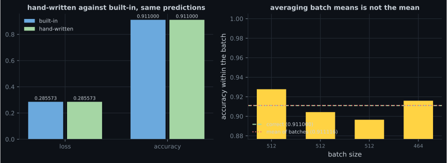
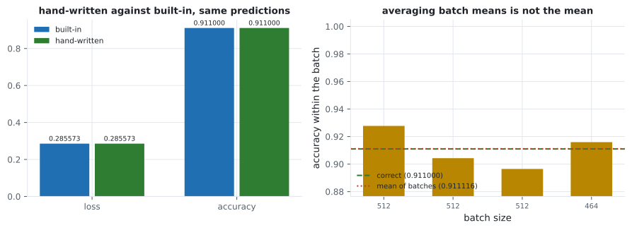
A loss must be differentiable, because Gradient Descent uses it. A metric just needs to be interpretable by a human, and doesn’t need a gradient. Most of the time you can reuse the same function for both — but not always. Consider precision over two batches: 4/5 correct in batch one (80%), 0/3 correct in batch two (0%). Averaging those two numbers gives 40%, but the real precision across both batches is 4/8 = 50%. A metric like this needs to accumulate counts across batches rather than average per-batch results — that’s a streaming metric, built by subclassing keras.metrics.Metrickeras.metrics.Metric:

A streaming metric that accumulates state

class HuberMetric(tf.keras.metrics.Metric):
    def __init__(self, threshold=1.0, **kwargs):
        super().__init__(**kwargs)
        self.threshold = threshold
        self.huber_fn = lambda yt, yp: huber_fn(yt, yp)
        self.total = self.add_weight("total", initializer="zeros")
        self.count = self.add_weight("count", initializer="zeros")
 
    def update_state(self, y_true, y_pred, sample_weight=None):
        metric = self.huber_fn(y_true, y_pred)
        self.total.assign_add(tf.reduce_sum(metric))
        self.count.assign_add(tf.cast(tf.size(y_true), tf.float32))
 
    def result(self):
        return self.total / self.count

A streaming metric that accumulates state

class HuberMetric(tf.keras.metrics.Metric):
    def __init__(self, threshold=1.0, **kwargs):
        super().__init__(**kwargs)
        self.threshold = threshold
        self.huber_fn = lambda yt, yp: huber_fn(yt, yp)
        self.total = self.add_weight("total", initializer="zeros")
        self.count = self.add_weight("count", initializer="zeros")
 
    def update_state(self, y_true, y_pred, sample_weight=None):
        metric = self.huber_fn(y_true, y_pred)
        self.total.assign_add(tf.reduce_sum(metric))
        self.count.assign_add(tf.cast(tf.size(y_true), tf.float32))
 
    def result(self):
        return self.total / self.count

add_weight()add_weight() creates the tracked variables (totaltotal, countcount); update_state()update_state() runs once per batch; result()result() returns the running mean whenever Keras asks for it.

Custom layers and models

A layer with no weights (like FlattenFlatten) is just a function wrapped in keras.layers.Lambdakeras.layers.Lambda. A layer with weights subclasses keras.layers.Layerkeras.layers.Layer:

A simplified Dense layer from scratch

class MyDense(tf.keras.layers.Layer):
    def __init__(self, units, activation=None, **kwargs):
        super().__init__(**kwargs)
        self.units = units
        self.activation = tf.keras.activations.get(activation)
 
    def build(self, batch_input_shape):
        self.kernel = self.add_weight(
            name="kernel", shape=[batch_input_shape[-1], self.units],
            initializer="glorot_normal")
        self.bias = self.add_weight(
            name="bias", shape=[self.units], initializer="zeros")
        super().build(batch_input_shape)
 
    def call(self, X):
        return self.activation(X @ self.kernel + self.bias)

A simplified Dense layer from scratch

class MyDense(tf.keras.layers.Layer):
    def __init__(self, units, activation=None, **kwargs):
        super().__init__(**kwargs)
        self.units = units
        self.activation = tf.keras.activations.get(activation)
 
    def build(self, batch_input_shape):
        self.kernel = self.add_weight(
            name="kernel", shape=[batch_input_shape[-1], self.units],
            initializer="glorot_normal")
        self.bias = self.add_weight(
            name="bias", shape=[self.units], initializer="zeros")
        super().build(batch_input_shape)
 
    def call(self, X):
        return self.activation(X @ self.kernel + self.bias)

build()build() runs once, the first time the layer sees an input, so it knows the input shape before creating the weight matrix. call()call() runs the actual computation every time the layer is used.

A model built by subclassing keras.Modelkeras.Model is the same idea, one level up — you create layers in __init__()__init__() and wire them together in call()call(), which lets you express skip connections and loops that the Sequential API can’t:

A model with a residual (skip-connection) block

class ResidualBlock(tf.keras.layers.Layer):
    def __init__(self, n_layers, n_neurons, **kwargs):
        super().__init__(**kwargs)
        self.hidden = [tf.keras.layers.Dense(n_neurons, activation="elu",
                                              kernel_initializer="he_normal")
                       for _ in range(n_layers)]
 
    def call(self, inputs):
        Z = inputs
        for layer in self.hidden:
            Z = layer(Z)
        return inputs + Z  # the skip connection
 
class ResidualRegressor(tf.keras.Model):
    def __init__(self, output_dim, **kwargs):
        super().__init__(**kwargs)
        self.hidden1 = tf.keras.layers.Dense(30, activation="elu",
                                              kernel_initializer="he_normal")
        self.block = ResidualBlock(2, 30)
        self.out = tf.keras.layers.Dense(output_dim)
 
    def call(self, inputs):
        Z = self.hidden1(inputs)
        for _ in range(4):
            Z = self.block(Z)  # reuse the same block 4 times
        return self.out(Z)

A model with a residual (skip-connection) block

class ResidualBlock(tf.keras.layers.Layer):
    def __init__(self, n_layers, n_neurons, **kwargs):
        super().__init__(**kwargs)
        self.hidden = [tf.keras.layers.Dense(n_neurons, activation="elu",
                                              kernel_initializer="he_normal")
                       for _ in range(n_layers)]
 
    def call(self, inputs):
        Z = inputs
        for layer in self.hidden:
            Z = layer(Z)
        return inputs + Z  # the skip connection
 
class ResidualRegressor(tf.keras.Model):
    def __init__(self, output_dim, **kwargs):
        super().__init__(**kwargs)
        self.hidden1 = tf.keras.layers.Dense(30, activation="elu",
                                              kernel_initializer="he_normal")
        self.block = ResidualBlock(2, 30)
        self.out = tf.keras.layers.Dense(output_dim)
 
    def call(self, inputs):
        Z = self.hidden1(inputs)
        for _ in range(4):
            Z = self.block(Z)  # reuse the same block 4 times
        return self.out(Z)

ModelModel is a subclass of LayerLayer, plus compile()compile(), fit()fit(), evaluate()evaluate(), and save()save(). As a rule of thumb: reusable building blocks subclass LayerLayer; the thing you actually train subclasses ModelModel.

Computing gradients with autodiff

Before writing a training loop by hand, you need a way to compute gradients. Analytically deriving them for a network with tens of thousands of parameters isn’t practical, and numerically approximating them (nudging each parameter a tiny amount and re-running the model) requires one full pass per parameter. TensorFlow’s autodiff needs only one forward pass and one backward pass, no matter how many parameters there are:

tf.GradientTape records operations, then computes gradients

def f(w1, w2):
    return 3 * w1 ** 2 + 2 * w1 * w2
 
w1, w2 = tf.Variable(5.), tf.Variable(3.)
with tf.GradientTape() as tape:
    z = f(w1, w2)
 
gradients = tape.gradient(z, [w1, w2])
print([g.numpy() for g in gradients])
# [36.0, 10.0]

tf.GradientTape records operations, then computes gradients

def f(w1, w2):
    return 3 * w1 ** 2 + 2 * w1 * w2
 
w1, w2 = tf.Variable(5.), tf.Variable(3.)
with tf.GradientTape() as tape:
    z = f(w1, w2)
 
gradients = tape.gradient(z, [w1, w2])
print([g.numpy() for g in gradients])
# [36.0, 10.0]

GradientTapeGradientTape watches every operation that touches a tf.Variabletf.Variable while its withwith block runs, then replays that record backward to compute derivatives. The tape is erased the moment you call .gradient().gradient() — pass persistent=Truepersistent=True if you need to call it more than once, and del tapedel tape afterward to free it.

diagram One custom training step mermaid

  flowchart LR
  A["Sample a batch (X, y)"] --> B["Forward pass: y_pred = model(X)"]
  B --> C["Compute loss(y, y_pred)"]
  C --> D["tape.gradient(loss, trainable_variables)"]
  D --> E["optimizer.apply_gradients(...)"]
  E --> A

How GradientTape turns a forward pass into a parameter update.

Writing a custom training loop

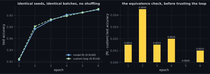
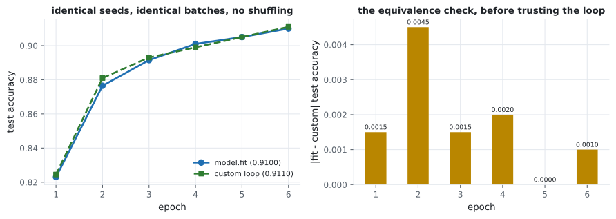
Most of the time, fit()fit() does exactly this loop for you. But if you need two optimizers for two parts of a network, or you just want to see every step happen explicitly, you can write it yourself:

A minimal custom training loop

import numpy as np
import tensorflow as tf
 
model = tf.keras.models.Sequential([
    tf.keras.layers.Dense(30, activation="elu", kernel_initializer="he_normal"),
    tf.keras.layers.Dense(1),
])
 
n_epochs = 5
batch_size = 32
optimizer = tf.keras.optimizers.Nadam(learning_rate=0.01)
loss_fn = tf.keras.losses.mean_squared_error
mean_loss = tf.keras.metrics.Mean()
 
def random_batch(X, y, batch_size=32):
    idx = np.random.randint(len(X), size=batch_size)
    return X[idx], y[idx]
 
for epoch in range(1, n_epochs + 1):
    for step in range(1, len(X_train) // batch_size + 1):
        X_batch, y_batch = random_batch(X_train, y_train, batch_size)
        with tf.GradientTape() as tape:
            y_pred = model(X_batch, training=True)
            main_loss = tf.reduce_mean(loss_fn(y_batch, y_pred))
            loss = tf.add_n([main_loss] + model.losses)  # + any regularization losses
        gradients = tape.gradient(loss, model.trainable_variables)
        optimizer.apply_gradients(zip(gradients, model.trainable_variables))
        mean_loss(loss)
    print(f"Epoch {epoch}: mean loss = {mean_loss.result():.4f}")
    mean_loss.reset_states()

A minimal custom training loop

import numpy as np
import tensorflow as tf
 
model = tf.keras.models.Sequential([
    tf.keras.layers.Dense(30, activation="elu", kernel_initializer="he_normal"),
    tf.keras.layers.Dense(1),
])
 
n_epochs = 5
batch_size = 32
optimizer = tf.keras.optimizers.Nadam(learning_rate=0.01)
loss_fn = tf.keras.losses.mean_squared_error
mean_loss = tf.keras.metrics.Mean()
 
def random_batch(X, y, batch_size=32):
    idx = np.random.randint(len(X), size=batch_size)
    return X[idx], y[idx]
 
for epoch in range(1, n_epochs + 1):
    for step in range(1, len(X_train) // batch_size + 1):
        X_batch, y_batch = random_batch(X_train, y_train, batch_size)
        with tf.GradientTape() as tape:
            y_pred = model(X_batch, training=True)
            main_loss = tf.reduce_mean(loss_fn(y_batch, y_pred))
            loss = tf.add_n([main_loss] + model.losses)  # + any regularization losses
        gradients = tape.gradient(loss, model.trainable_variables)
        optimizer.apply_gradients(zip(gradients, model.trainable_variables))
        mean_loss(loss)
    print(f"Epoch {epoch}: mean loss = {mean_loss.result():.4f}")
    mean_loss.reset_states()

Notice model(X_batch, training=True)model(X_batch, training=True) — layers like DropoutDropout or BatchNormalizationBatchNormalization behave differently at train vs. test time, so you must pass training=Truetraining=True yourself; fit()fit() normally does this for you. This loop also skips weight constraints and doesn’t handle per-batch validation — a real custom loop needs a few more lines for those. That’s the trade-off: full control, at the cost of writing (and debugging) more code yourself.

Speeding it up with tf.function

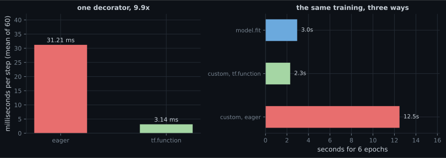
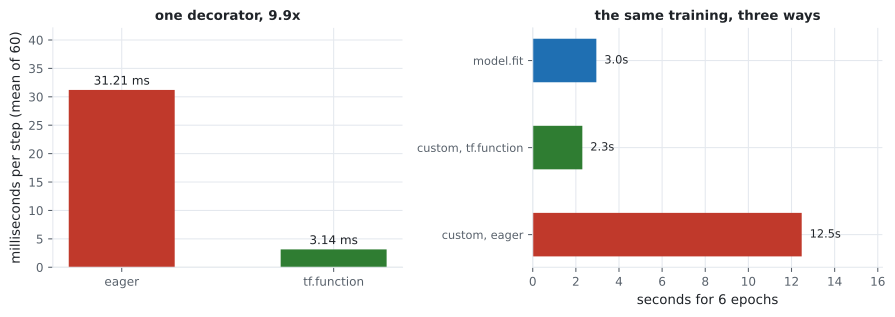
Wrapping a Python function in @tf.function@tf.function lets TensorFlow trace it once into an optimized computation graph, then reuse that graph on every call — often much faster than re-running the raw Python:

Turning a Python function into a TF Function

@tf.function
def train_step(X_batch, y_batch):
    with tf.GradientTape() as tape:
        y_pred = model(X_batch, training=True)
        loss = tf.reduce_mean(loss_fn(y_batch, y_pred))
    gradients = tape.gradient(loss, model.trainable_variables)
    optimizer.apply_gradients(zip(gradients, model.trainable_variables))
    return loss

Turning a Python function into a TF Function

@tf.function
def train_step(X_batch, y_batch):
    with tf.GradientTape() as tape:
        y_pred = model(X_batch, training=True)
        loss = tf.reduce_mean(loss_fn(y_batch, y_pred))
    gradients = tape.gradient(loss, model.trainable_variables)
    optimizer.apply_gradients(zip(gradients, model.trainable_variables))
    return loss

When you use a custom loss, metric, or layer inside a tf.kerastf.keras model, Keras converts it to a TF Function automatically — you rarely need to reach for @tf.function@tf.function yourself unless you’re writing a fully manual loop like the one above.

A note on mixed precision in a custom loop

fit()fit() handles one more detail automatically that a hand-rolled loop doesn’t: if you’ve turned on a mixed-precision policy (see Mixed Precision and Multi-GPU Training), very small gradient values computed in float16 can underflow to zero before they ever reach the optimizer. fit()fit() quietly wraps your optimizer to guard against this; in a custom loop you need to do it yourself by wrapping the optimizer in a LossScaleOptimizerLossScaleOptimizer, which temporarily scales the loss up before computing gradients and scales the resulting gradients back down before applying them:

Loss scaling for mixed precision in a custom loop

optimizer = tf.keras.optimizers.Nadam(learning_rate=0.01)
optimizer = tf.keras.mixed_precision.LossScaleOptimizer(optimizer)
 
with tf.GradientTape() as tape:
    y_pred = model(X_batch, training=True)
    loss = loss_fn(y_batch, y_pred)
    scaled_loss = optimizer.get_scaled_loss(loss)
 
scaled_gradients = tape.gradient(scaled_loss, model.trainable_variables)
gradients = optimizer.get_unscaled_gradients(scaled_gradients)
optimizer.apply_gradients(zip(gradients, model.trainable_variables))

Loss scaling for mixed precision in a custom loop

optimizer = tf.keras.optimizers.Nadam(learning_rate=0.01)
optimizer = tf.keras.mixed_precision.LossScaleOptimizer(optimizer)
 
with tf.GradientTape() as tape:
    y_pred = model(X_batch, training=True)
    loss = loss_fn(y_batch, y_pred)
    scaled_loss = optimizer.get_scaled_loss(loss)
 
scaled_gradients = tape.gradient(scaled_loss, model.trainable_variables)
gradients = optimizer.get_unscaled_gradients(scaled_gradients)
optimizer.apply_gradients(zip(gradients, model.trainable_variables))

One more reason, alongside everything above, that Géron recommends reaching for fit()fit() whenever you can.

Mini-checkpoint

Custom loss, differentiable, drives training → plain function, or subclass keras.losses.Losskeras.losses.Loss if it has hyperparameters to save.
Custom metric, human-readable, can be non-differentiable → plain function if it averages cleanly per batch, or subclass keras.metrics.Metrickeras.metrics.Metric if it needs to accumulate state (like precision).
tape.gradient(loss, trainable_variables)tape.gradient(loss, trainable_variables) + optimizer.apply_gradients(...)optimizer.apply_gradients(...) is the two-line heart of every training loop, custom or not.

🧪 Try It Yourself

Exercise 1 – Write the Huber loss with tf.where

Exercise 2 – Compute gradients with GradientTape

Exercise 3 – Apply gradients in a training step

Continue to Distributed Training with tf.distribute — once you can train a model with a custom loop on one device, the next step is spreading that same training across many GPUs (or machines) at once.

If this helped you, consider buying me a coffee ☕

Buy me a coffee