Feature Scaling (Normalization & Standardization)

What you’ll learn

• the three scaler formulas, each computed by hand on the same five numbers
• which models are destroyed by unscaled features, which are indifferent, and why — measured
• what a single outlier does to each scaler, quantified
• why fit belongs to the training set and transform to everything
• when to log-transform instead of scale
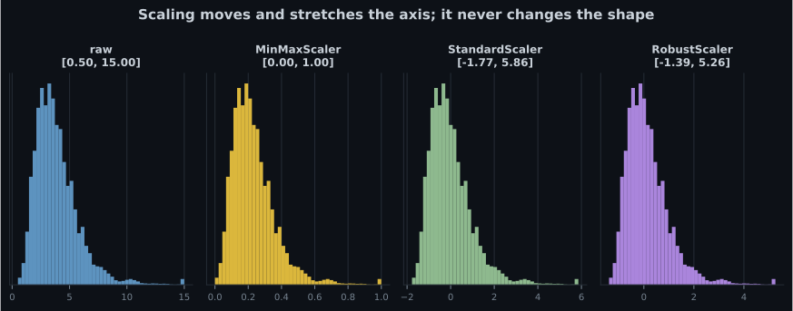
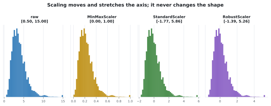
• that scaling never changes the shape of a distribution

Intuition

The housing data has median_income spanning 0.5 to 15 and population spanning 3 to 35,682. Nothing is wrong with either column. The problem is that some algorithms treat “a difference of 1” as meaning the same thing in both.

Two model families care intensely:

• Distance-based — KNN, SVM with RBF, k-means. Euclidean distance sums squared differences, so a feature with a range in the thousands drowns one with a range of 10.
• Gradient-based — linear and logistic regression via SGD, neural networks. Unequal feature scales stretch the cost surface into a ravine, and descent zig-zags instead of descending.

Two families do not:

• Tree-based — splits depend on the ordering of values, and scaling is monotone.
• Closed-form solvers — the Normal Equation solves exactly regardless of conditioning, within numerical limits.

diagram Diagram mermaid

  flowchart TD
  A["Feature ranges differ
by orders of magnitude"] --> B{"How does the model
use the numbers?"}
  B -->|"distances"| C["KNN, SVM, k-means
SCALING REQUIRED"]
  B -->|"iterative gradients"| D["SGD, neural networks
SCALING REQUIRED"]
  B -->|"value ordering"| E["Trees, forests, boosting
no effect"]
  B -->|"closed form"| F["Normal Equation
no effect"]

The math

$$x_{\text{minmax}} = \frac{x - \min(x)}{\max(x) - \min(x)} \qquad x_{\text{std}} = \frac{x - \mu}{\sigma} \qquad x_{\text{robust}} = \frac{x - \text{median}(x)}{Q_3 - Q_1}$$

Scaler	Centre	Spread	Output range	Outlier behaviour
MinMaxScaler	min	range	exactly $[0, 1]$	Terrible — one point sets the range
StandardScaler	mean	std	unbounded, mean 0, sd 1	Poor — both statistics move
RobustScaler	median	IQR	unbounded	Good — both statistics resist

StandardScaler uses the population standard deviation ($\div n$, not $\div (n-1)$), which is why hand calculations must use $\sigma$ rather than pandas’ default $s$.

Worked example by hand

Five values: $[1, 2, 3, 4, 5]$.

Step 1 — the statistics.

$$\min = 1,\quad \max = 5,\quad \mu = 3,\quad \sigma = \sqrt{\tfrac{4+1+0+1+4}{5}} = \sqrt{2} \approx 1.4142,\quad Q_1 = 2,\; \text{median} = 3,\; Q_3 = 4$$

Step 2 — apply each formula.

$x$	min-max $\frac{x-1}{4}$	standard $\frac{x-3}{1.4142}$	robust $\frac{x-3}{2}$
1	0.00	−1.4142	−1.0
2	0.25	−0.7071	−0.5
3	0.50	0.0000	0.0
4	0.75	0.7071	0.5
5	1.00	1.4142	1.0

Step 3 — check the properties. Min-max lands exactly on $[0, 1]$. Standardised values have mean 0 and population standard deviation 1. Robust values are centred on the median with the interquartile range as the unit.

Step 4 — note what did not change. All three columns are perfectly evenly spaced, exactly as the original was. Scaling is an affine map: it slides and stretches the axis and can do nothing else.

figure The same column, four treatments matplotlib

The right-skew survives every scaler unchanged. If you wanted to fix the skew you needed a log, not a scaler.

What one outlier does

figure Values 1 to 10, plus one reading of 1000 matplotlib

Min-max crushes the ten real values into a span of 0.009 — they are now numerically indistinguishable. RobustScaler keeps them spread over 1.8 and lets the outlier fly off to 198.8.

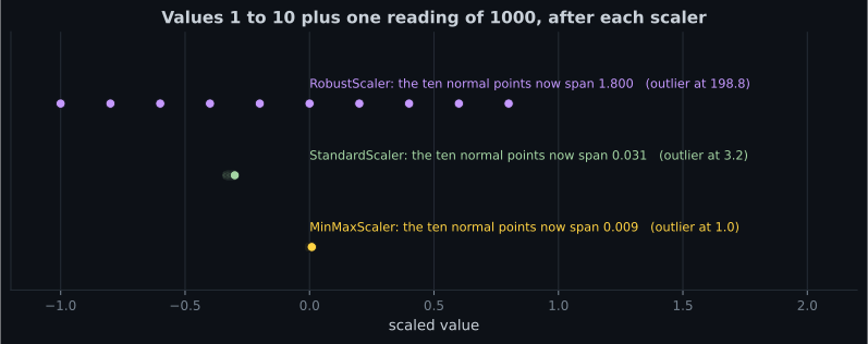
Reading the plot

Scaler	Span of the ten normal values	Where the outlier lands
MinMaxScaler	0.0090	1.000
StandardScaler	0.0315	3.162
RobustScaler	1.8000	198.800

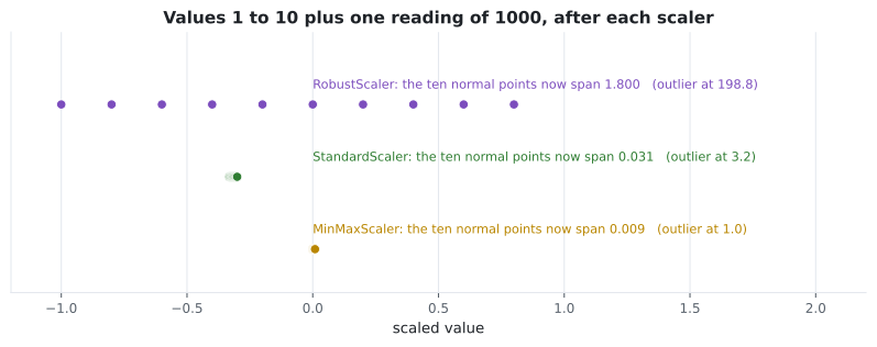
1. Min-max is catastrophic. The single value of 1000 defines the range, so the ten real observations occupy 0.9% of the output interval. Any distance computed between them is now effectively zero.
2. Standardisation is bad but less so. The outlier inflates $\sigma$, compressing everything else into a span of 0.03.
3. RobustScaler keeps the real data readable. Median and IQR ignore the extreme value entirely, so the ten normal points keep a usable spread — and the outlier is left at 198.8, visibly flagged rather than silently absorbed.

RobustScaler is the right default whenever outliers are present and cannot be removed.

See it move

Two features, wildly different ranges. Watch the cloud transform as the scalers are applied — and watch the shape stay exactly where it was.

sketch Scaling moves the axes, not the data p5.js Pause Restart

A cloud of points with one feature spanning thousands and the other spanning tens, cycling through raw, min-max, standardised and robust scaling. The relative arrangement of the points never changes.

Which models actually care

figure Five models, with and without scaling matplotlib

SGD on raw features diverges to an RMSE of about 3.8 quadrillion. KNN improves by 31%. Linear regression, SVR and the random forest are essentially unchanged.

who_cares.py

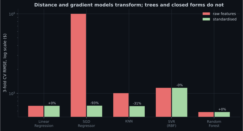
import numpy as np
import pandas as pd
from sklearn.ensemble import RandomForestRegressor
from sklearn.linear_model import LinearRegression, SGDRegressor
from sklearn.model_selection import cross_val_score
from sklearn.neighbors import KNeighborsRegressor
from sklearn.pipeline import make_pipeline
from sklearn.preprocessing import StandardScaler
from sklearn.svm import SVR
 
housing = pd.read_csv(URL).dropna()
X = housing.select_dtypes("number").drop(columns=["median_house_value"]).values
y = housing["median_house_value"].values
sample = np.random.default_rng(0).choice(len(y), 3000, replace=False)
X, y = X[sample], y[sample]
 
models = {
    "linear": LinearRegression(),
    "sgd": SGDRegressor(max_iter=2000, tol=1e-4, random_state=0),
    "knn": KNeighborsRegressor(10),
    "svr": SVR(),
    "forest": RandomForestRegressor(n_estimators=60, random_state=0, n_jobs=-1),
}
 
for name, model in models.items():
    raw = -cross_val_score(model, X, y, cv=3,
                           scoring="neg_root_mean_squared_error").mean()
    scaled = -cross_val_score(make_pipeline(StandardScaler(), model), X, y, cv=3,
                              scoring="neg_root_mean_squared_error").mean()
    print(f"{name:<7} raw {raw:>22,.0f}   scaled {scaled:>9,.0f}   "
          f"{100 * (scaled - raw) / raw:+7.1f}%")
 
# linear  raw                 69,721   scaled    69,721      +0.0%
# sgd     raw  3,795,293,450,055,030   scaled    70,035    -100.0%
# knn     raw                100,607   scaled    69,128     -31.3%
# svr     raw                117,412   scaled   117,374      -0.0%
# forest  raw                 58,226   scaled    58,263      +0.1%

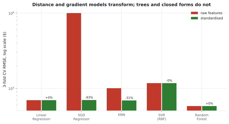
Reading the table

• SGD is the headline. Raw features produce an RMSE of $3.8 \times 10^{15}$ — the optimiser diverged. Scaling turns a broken model into a working one, matching the closed-form solution to within 0.5%. Not an improvement; a repair.
• KNN gains 31%. Distance was being dominated by population, which spans 35,000, while median_income spanning 15 contributed almost nothing.
• Linear regression is byte-identical. LinearRegression uses lstsq, and least squares is invariant to affine feature transformations.
• The forest is unchanged to within noise, exactly as the theory says.
• SVR barely moves here only because this sample happens to be dominated by one large-range feature either way; on the full dataset with an RBF kernel, scaling matters a great deal.

Fit on train, transform everything

fit_on_train.py

from sklearn.model_selection import train_test_split
from sklearn.preprocessing import StandardScaler
 
X_train, X_test = train_test_split(X, test_size=0.2, random_state=42)
 
scaler = StandardScaler()
scaler.fit(X_train)                    # learn mu and sigma from training data only
 
X_train_scaled = scaler.transform(X_train)
X_test_scaled = scaler.transform(X_test)     # NOT fit_transform
 
print(X_train_scaled.mean(axis=0).round(6))  # ~0 by construction
print(X_test_scaled.mean(axis=0).round(4))   # near 0, but not exactly — correct

The test set’s scaled mean is not exactly zero, and that is the point. It was scaled by parameters learned elsewhere, exactly as a live request will be. If your test data scales to a perfect mean of zero, you called fit_transform on it and leaked.

fit_transform on the test set

The most common leak in preprocessing. scaler.fit_transform(X_test) computes the test set’s own mean and standard deviation — statistics that will not exist when a single row arrives in production. The reported score becomes unreproducible in the real world. Put the scaler in a Pipeline and the mistake becomes impossible to make.

Scaling is not transforming

Scaling cannot fix skew, because it is affine. Six of the nine housing columns are heavily right-skewed, and no scaler touches that. A logarithm does:

log_transform.py

import numpy as np
from scipy import stats
 
col = housing["population"]
print("raw skew:", round(float(stats.skew(col)), 3))            # 4.935
print("scaled skew:", round(float(stats.skew(
    (col - col.mean()) / col.std())), 3))                       # 4.935 — unchanged
print("log skew:", round(float(stats.skew(np.log1p(col))), 3))  # -1.044

Standardising leaves the skew at 4.94. log1p brings it to −1.04 — overshooting into a mild left skew, which is a reminder that a log is a fixed transform, not a tuned one. Different tools for different problems: scalers equalise ranges, transforms reshape distributions.

Situation	Reach for
Features on different scales, no outliers	StandardScaler
Outliers present	RobustScaler
Bounded input required (image pixels, some neural nets)	MinMaxScaler
Heavy right skew	np.log1p, then a scaler
Skew of unknown form	PowerTransformer(method="yeo-johnson")
Only the rank matters	QuantileTransformer

Pitfalls

Scaling before splitting

StandardScaler().fit_transform(X) on the full dataset computes a mean that includes test rows. Split first, or use a pipeline.

Scaling the target without inverting

Scaling y is legitimate — it can help gradient methods converge. But predict() then returns scaled values, and reporting an RMSE of 0.31 in standard-deviation units is meaningless to a stakeholder. Use TransformedTargetRegressor, which inverts automatically.

Scaling one-hot columns

Standardising a 0/1 column produces values like −0.42 and 2.37, which is harmless but destroys the readability of coefficients and importances. Scale numeric columns only — which is exactly what ColumnTransformer is for.

Assuming a scaler fixed your outliers

MinMaxScaler maps everything into $[0, 1]$, and the outlier is still there at 1.0 with everything else crushed near 0. Detect and handle outliers separately; scaling only relabels the axis.

pch.quizTag pch.quizDefaultTitle

1. Why does scaling not affect a decision tree?

   A Trees rescale internally B A split tests whether a value is above or below a threshold, and any monotone rescaling preserves that ordering C Trees only use categorical features D It does affect them; not scaling is a common mistake
   pch.quizShowAnswer

   B — A split tests whether a value is above or below a threshold, and any monotone rescaling preserves that ordering — Scaling is monotone, so it maps every threshold to a corresponding threshold. The partition of the data — and therefore the tree — is identical.

2. MinMaxScaler is applied to values 1 to 10 plus one reading of 1000. What happens to the ten normal values?

   A They spread evenly across 0 to 1 B They are compressed into a span of about 0.009, because the outlier defines the entire range C They are removed as outliers D They become negative
   pch.quizShowAnswer

   B — They are compressed into a span of about 0.009, because the outlier defines the entire range — Min-max divides by max minus min, which the outlier sets to 999. The real data occupies 0.9% of the output interval and becomes numerically indistinguishable.

3. Why must you call transform, not fit_transform, on the test set?

   A fit_transform is slower B Fitting on test data uses statistics that will not exist at prediction time, so the reported score cannot be reproduced in production C It would raise an error D There is no difference between them
   pch.quizShowAnswer

   B — Fitting on test data uses statistics that will not exist at prediction time, so the reported score cannot be reproduced in production — A single live request has no mean or standard deviation of its own. The scaler must replay the parameters it learned during training, and the test set has to be treated the same way.

4. Your feature has a skew of 4.94. You standardise it. What is the new skew?

   A 0.00 B About 1.00 C 4.94 — unchanged D Negative
   pch.quizShowAnswer

   C — 4.94 — unchanged — Standardisation is an affine map: subtract a constant, divide by a constant. Skewness is invariant to both. Use a log or a power transform to change the shape.

🧪 Try It Yourself

Exercise 1 – Min-max scale by hand

pch.exerciseTag pch.exerciseTitle

Exercise 2 – Standardise, and match scikit-learn

pch.exerciseTag pch.exerciseTitle

Exercise 3 – Watch one outlier crush the rest

pch.exerciseTag pch.exerciseTitle

Exercise 4 – Fit on train, transform both

pch.exerciseTag pch.exerciseTitle

Exercise 5 – Scaling cannot fix skew

pch.exerciseTag pch.exerciseTitle

Recap

• Min-max maps to $[0,1]$, standardisation to mean 0 and sd 1, robust to median 0 and IQR 1.
• Worked by hand on $[1,2,3,4,5]$: all three produce evenly spaced output, because scaling is affine.
• Distance-based and gradient-based models need scaling; trees and closed-form solvers do not. SGD on raw housing features reaches an RMSE of $3.8\times10^{15}$; scaled, it matches the exact solution.
• One outlier crushes the ten real values into a span of 0.009 under min-max and 0.032 under standardisation, against 1.8 under RobustScaler.
• Fit on train, transform on everything. A test set that scales to exactly zero mean is evidence of a leak.
• Scaling cannot change skewness — 4.935 before and after. Use log1p or PowerTransformer for that.

Exercise 6 – Which scaler survives one outlier?

pch.exerciseTag pch.exerciseTitle

Next

Continue to Transformation Pipelines & Custom Transformers — assemble imputing, encoding and scaling into one object that cannot leak.