Naïve Bayes Classifier

What you’ll learn

• Bayes’ theorem, and the base-rate trap that catches almost everyone
• what exactly is naive about Naive Bayes, and why the model works anyway
• a complete spam classification computed by hand, matching scikit-learn to four decimals
• Laplace smoothing — the one line that stops a single unseen word zeroing everything
• why log-space arithmetic is mandatory, not an optimisation
• Gaussian, Multinomial, Bernoulli and Complement variants, and which to reach for

Intuition

Every other classifier in this phase learns a boundary. Naive Bayes learns a story about how the data was generated, then asks which story best explains each new observation.

The story: a class was chosen, and then the features were drawn from that class’s distribution. To classify, invert the story — given these features, which class most likely produced them? That inversion is Bayes’ theorem.

What makes it naive is one simplification: given the class, all features are assumed independent. That is essentially always false. In text, “New” and “York” are wildly dependent. The model survives anyway, for a reason worth understanding.

diagram Diagram mermaid

  flowchart LR
  P["Prior
P(class)"] --> M["Multiply"]
  L["Likelihood
P(features | class)"] --> M
  M --> U["Unnormalised score
per class"]
  U --> N["Normalise across classes"]
  N --> POST["Posterior P(class | features)"]
  POST --> A["argmax = prediction"]

The math

Bayes’ theorem

$$P(A \mid B) = \frac{P(B \mid A)\,P(A)}{P(B)}$$

For classification, with class $c$ and feature vector $\mathbf{x}$:

$$P(c \mid \mathbf{x}) = \frac{P(\mathbf{x} \mid c)\,P(c)}{P(\mathbf{x})}$$

$P(\mathbf{x})$ is identical for every class, so it cannot affect which class wins:

$$\hat{y} = \operatorname*{arg\,max}_{c}\; P(c) \cdot P(\mathbf{x} \mid c)$$

Where this comes from

The derivation from the product rule, and the distinction between prior, likelihood, evidence and posterior, is in Sum Rule, Product Rule, and Bayes Theorem.

The naive assumption

$P(\mathbf{x} \mid c) = P(x_1, x_2, \ldots, x_n \mid c)$ is a joint distribution over every feature combination. With 1,000 binary features that is $2^{1000}$ parameters — unlearnable from any dataset. Assume conditional independence and the joint factorises into a product:

$$P(\mathbf{x} \mid c) = \prod_{j=1}^{n} P(x_j \mid c)$$ $$\boxed{\;\hat{y} = \operatorname*{arg\,max}_{c}\; P(c)\prod_{j=1}^{n} P(x_j \mid c)\;}$$

The parameter count collapses from exponential to linear. That is the entire trade: an assumption that is false, in exchange for a model that can actually be fitted — in one pass over the data, with no optimisation at all.

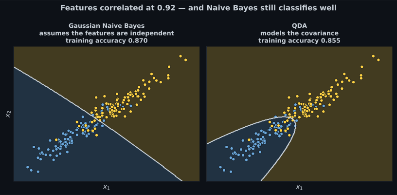
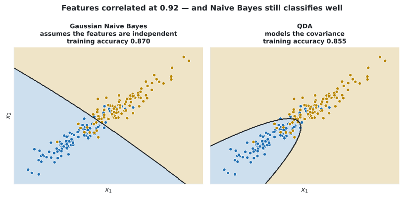
Why being wrong does not matter much

Naive Bayes usually produces badly calibrated probabilities and surprisingly good classifications. The two facts share a cause.

When features are correlated, multiplying their likelihoods double-counts the same evidence, so the posterior is pushed toward 0 or 1 far harder than the data justifies — outputs of 0.9999 are routine and rarely mean what they say. But classification only needs the arg max. Overstating the winning class’s score does not change which class wins. The ranking survives even when the numbers do not.

figure Features correlated at 0.92, and it barely matters matplotlib

Naive Bayes fits axis-aligned ellipses and cannot represent the tilt. QDA models the covariance properly. The boundaries differ visibly; the accuracies barely do.

Worked example by hand: the base-rate trap

Before the classifier, the intuition pump. A disease affects 1% of people. A test detects it 99% of the time and has a 5% false-positive rate. You test positive. What is the probability you have it?

Step 1 — write down what is known.

$$P(D) = 0.01,\quad P(+ \mid D) = 0.99,\quad P(+ \mid \neg D) = 0.05$$

Step 2 — total probability of a positive test.

$$P(+) = P(+ \mid D)P(D) + P(+ \mid \neg D)P(\neg D) = (0.99)(0.01) + (0.05)(0.99) = 0.0099 + 0.0495 = 0.0594$$

Step 3 — invert.

$$P(D \mid +) = \frac{(0.99)(0.01)}{0.0594} = \frac{0.0099}{0.0594} = 0.1667$$

About one in six. Most people guess 95% or higher. The reason is the base rate: healthy people outnumber sick ones 99 to 1, so even a 5% error rate among them produces five times more false positives than there are true positives. The prior is doing most of the work, and this is exactly what Naive Bayes formalises.

See it move

The arithmetic is three lines, so the useful thing to vary is the inputs. The sketch lays out 2,000 people as a grid, colours them by true status and test result, and reports $P(D \mid +)$ as the prevalence sweeps. The posterior is not a property of the test — it moves by more than a factor of ten while the test’s own numbers never change.

sketch The same test, four different answers p5.js Pause Restart

Two thousand people shown as a grid of squares, coloured as true positives, false positives, and everyone who tested negative. Prevalence sweeps from 0.1 percent to 20 percent while sensitivity and specificity stay fixed; the posterior probability of disease given a positive test tracks the prevalence, not the test. Click to pause.

Four readings from the same test, all computed with the same three numbers:

Prevalence	True positives	False positives	$P(D \mid +)$
0.1%	2	100	0.0196
1%	20	99	0.1681
5%	99	95	0.5103
20%	396	80	0.8319

Nothing about the test changed between the first row and the last, and its answer went from “almost certainly a false alarm” to “probably real”. This is why a screening tool validated on a high-prevalence clinical population misbehaves when it is rolled out to the general population, and why predict_proba from a model trained on resampled data cannot be read as a probability until the prior is put back.

Worked example by hand: a spam filter

Six training documents, three of each class.

Class	Documents
spam	“win money now” · “cheap money offer” · “win big prize money”
ham	“meeting at noon” · “project meeting notes” · “lunch meeting notes”

Step 1 — vocabulary and counts. The vocabulary has $V = 13$ distinct words.

	spam count	ham count
win	2	0
money	3	0
now	1	0
cheap	1	0
offer	1	0
big	1	0
prize	1	0
meeting	0	3
at	0	1
noon	0	1
project	0	1
notes	0	2
lunch	0	1
total words	10	9

Step 2 — priors. Three documents each, so $P(\text{spam}) = P(\text{ham}) = 0.5$.

Step 3 — likelihoods with Laplace smoothing. Add 1 to every count so nothing is impossible:

$$P(w \mid c) = \frac{\text{count}(w, c) + \alpha}{N_c + \alpha V}, \qquad \alpha = 1$$

Classify the new document “cheap prize money”:

$$P(\text{cheap} \mid \text{spam}) = \frac{1+1}{10+13} = \frac{2}{23} \quad P(\text{prize} \mid \text{spam}) = \frac{2}{23} \quad P(\text{money} \mid \text{spam}) = \frac{3+1}{23} = \frac{4}{23}$$ $$P(\text{cheap} \mid \text{ham}) = \frac{0+1}{9+13} = \frac{1}{22} \quad P(\text{prize} \mid \text{ham}) = \frac{1}{22} \quad P(\text{money} \mid \text{ham}) = \frac{1}{22}$$

Step 4 — multiply.

$$\text{score}_{\text{spam}} = 0.5 \times \frac{2}{23}\times\frac{2}{23}\times\frac{4}{23} = 0.5 \times \frac{16}{12167} = 6.575\times10^{-4}$$ $$\text{score}_{\text{ham}} = 0.5 \times \left(\frac{1}{22}\right)^{3} = 0.5 \times \frac{1}{10648} = 4.696\times10^{-5}$$

Step 5 — normalise.

$$P(\text{spam} \mid \text{doc}) = \frac{6.575\times10^{-4}}{6.575\times10^{-4} + 4.696\times10^{-5}} = 0.9333$$

MultinomialNB on the same six documents returns [0.0667, 0.9333] — the hand calculation to four decimal places.

Without smoothing this breaks completely

“cheap” never appears in a ham document, so the unsmoothed $P(\text{cheap} \mid \text{ham}) = 0$. One zero in the product makes the entire ham score zero, and the model becomes certain the document is spam on the strength of one unseen word. Laplace smoothing (alpha=1) is the default in scikit-learn for exactly this reason. Set alpha=0 and you will eventually hit it.

Log space is mandatory

Multiplying hundreds of probabilities underflows to zero in floating point. A 300-word document with typical word probabilities around $10^{-4}$ produces $10^{-1200}$, and float64 bottoms out near $10^{-308}$.

Take logarithms and products become sums:

$$\log P(c \mid \mathbf{x}) \propto \log P(c) + \sum_{j=1}^{n} \log P(x_j \mid c)$$

The arg max is unchanged, because the logarithm is monotonic. Every real implementation, including scikit-learn’s predict_log_proba, works this way. This is not an optimisation — without it, long documents produce zero for every class and the classifier returns whichever comes first.

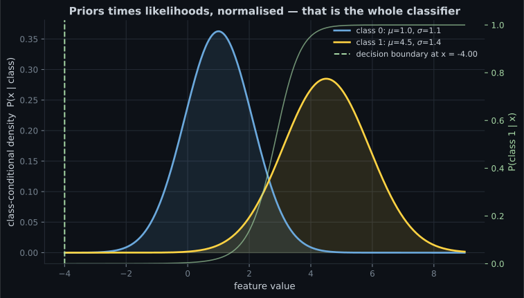
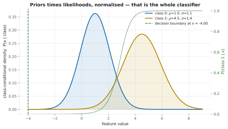
The Gaussian variant

For continuous features, model each feature within each class as a normal distribution, estimating $\mu_{jc}$ and $\sigma_{jc}$ from the training data:

$$P(x_j \mid c) = \frac{1}{\sqrt{2\pi\sigma_{jc}^{2}}}\exp\left(-\frac{(x_j - \mu_{jc})^2}{2\sigma_{jc}^{2}}\right)$$

Fitting is just computing a mean and a variance per feature per class — one pass, no iteration, no hyperparameters.

figure What GaussianNB actually stores matplotlib

Two numbers per class per feature. The boundary sits where prior times likelihood is equal for both classes — not where the curves themselves cross, because the priors differ.

Reading the plot

• The boundary is not the midpoint of the two means. Class 0 has the higher prior (0.6), which pushes the crossing point toward class 1’s territory.
• The posterior curve is a sigmoid. For two Gaussians with equal variance, Gaussian Naive Bayes produces exactly the logistic function — the same S-curve as logistic regression, reached from entirely different assumptions.
• The shape is decided by the variances, which is what makes this a generative model: it can also sample new data, something logistic regression cannot do.

Choosing a variant

Variant	Feature type	Classic use	scikit-learn
Gaussian	Continuous	Sensor readings, measurements	GaussianNB
Multinomial	Counts	Word counts, TF-IDF	MultinomialNB
Bernoulli	Binary	Word present / absent, short texts	BernoulliNB
Complement	Counts, imbalanced	Text with very uneven class sizes	ComplementNB
Categorical	Discrete categories	Survey answers, encoded categoricals	CategoricalNB

ComplementNB is worth knowing: it estimates each class’s parameters from the complement of that class, which corrects the bias MultinomialNB develops when one class dominates the corpus.

text_classification.py

from sklearn.feature_extraction.text import CountVectorizer
from sklearn.naive_bayes import MultinomialNB
 
docs = [
    "win money now", "cheap money offer", "win big prize money",
    "meeting at noon", "project meeting notes", "lunch meeting notes",
]
labels = [1, 1, 1, 0, 0, 0]        # 1 = spam
 
vectoriser = CountVectorizer()
X = vectoriser.fit_transform(docs)
print(f"vocabulary size: {len(vectoriser.vocabulary_)}")   # 13
 
model = MultinomialNB(alpha=1.0).fit(X, labels)
 
test = vectoriser.transform(["cheap prize money"])
print(model.predict_proba(test).round(4))    # [[0.0667 0.9333]]
print(model.predict(test))                   # [1]

Identical to the hand calculation, which is the point of doing both.

gaussian_nb.py

from sklearn.datasets import load_breast_cancer
from sklearn.model_selection import train_test_split
from sklearn.naive_bayes import GaussianNB
 
X, y = load_breast_cancer(return_X_y=True)
y = 1 - y
X_tr, X_te, y_tr, y_te = train_test_split(
    X, y, test_size=0.3, random_state=0, stratify=y
)
 
model = GaussianNB().fit(X_tr, y_tr)
 
print(f"test accuracy {model.score(X_te, y_te):.4f}")   # 0.9123
print(f"class priors  {model.class_prior_.round(4)}")   # [0.6281 0.3719]
print(f"parameters stored: {model.theta_.shape}")       # (2, 30) means + variances

91% accuracy on 30 correlated medical features, from a model that assumes they are all independent and that trains in a single pass. Logistic regression reaches 95% on the same split — better, but it needed an iterative solver and scaling to get there.

pch.algoTag Naive Bayes Supervised · Classification · Generative

pch.algoApi sklearn.naive_bayes.GaussianNB / MultinomialNB / BernoulliNB / ComplementNB

pch.algoAssumes

• Features are conditionally independent given the class — almost always false, and usually survivable
• The chosen likelihood matches the data: Gaussian for continuous, multinomial for counts
• Training class frequencies reflect the deployment priors, unless you override them

pch.algoCost

pch.algoTrain

O(m·n) — one pass

pch.algoPredict

O(n·K)

pch.algoMemory

O(n·K)

m = samples, n = features, K = classes

pch.algoHyperparams

• alpha default 1.0 Laplace/Lidstone smoothing for the count-based variants. Never set it to 0 unless every word is guaranteed to appear in every class.
• fit_prior default True Estimate class priors from the training data. Set False for a uniform prior when training frequencies are an artefact of collection.
• class_prior default None Supply real-world priors directly — valuable when the training set was deliberately balanced but production is not.
• var_smoothing default 1e-9 (GaussianNB) Added to every variance for stability. Raise it if a feature is near-constant within a class.

pch.algoReachFor

• Text classification — it remains a genuinely strong baseline
• Very high-dimensional sparse data
• You need a model trained in seconds on millions of rows
• Data arrives in a stream — partial_fit supports online updates

pch.algoLookElsewhere

• You need well-calibrated probabilities
• Features are strongly dependent and you need the boundary to reflect it
• There are few features and plenty of data — a discriminative model will beat it
• Continuous features are strongly non-Gaussian and cannot be transformed

Pitfalls

alpha=0 and the zero-frequency problem

One unseen word makes the entire product zero for that class, and the model becomes certain on the strength of a single token. Keep alpha=1, or tune it in the range 0.01 to 1 — never zero.

The probabilities are not trustworthy

Correlated features double-count evidence, so posteriors get pushed to 0.9999 and 0.0001 far too readily. Fine for ranking or arg max, unsafe for anything that consumes the number itself. Wrap in CalibratedClassifierCV if you need honest probabilities.

Match the variant to the data

GaussianNB on word counts assumes counts are normally distributed, which they are not — counts are non-negative, integer, and heavily skewed. MultinomialNB on standardised continuous features fails too, since it expects non-negative values. Choosing the wrong variant is the most common Naive Bayes bug.

Training priors may not be deployment priors

If you balanced the training set by downsampling the majority class, the learned priors are wrong for production. Pass real-world priors via class_prior, or set fit_prior=False.

Compare

Model	Type	Training cost	Probabilities	Handles correlated features
Naive Bayes	Generative	One pass, $O(m \cdot n)$	Poorly calibrated	Assumes they are not
Logistic Regression	Discriminative	Iterative	Well calibrated	Yes
Linear SVM	Discriminative	Quadratic program	Needs Platt scaling	Yes
Random Forest	Discriminative	Moderate	Reasonable	Yes

The generative/discriminative distinction is the deep one. Naive Bayes models $P(\mathbf{x} \mid c)$ and can therefore generate new samples; logistic regression models $P(c \mid \mathbf{x})$ directly and cannot. Modelling less is usually the better bet for pure classification accuracy — but it costs you the ability to ask “what does a typical spam email look like?”

pch.quizTag pch.quizDefaultTitle

1. A disease affects 1% of people. A test is 99% sensitive with a 5% false-positive rate. You test positive. Roughly what is the probability you have the disease?

   A 99% B 95% C 17% D 1%
   pch.quizShowAnswer

   C — 17% — P(D|+) = 0.0099 / 0.0594 = 0.167, about one in six. Healthy people outnumber sick ones 99 to 1, so 5% of them produces five times more false positives than there are true positives.

2. What exactly is 'naive' about Naive Bayes?

   A It uses a very simple optimisation algorithm B It assumes every feature is independent of the others given the class, which collapses an exponential joint distribution into a product C It assumes all classes are equally likely D It assumes the data is Gaussian
   pch.quizShowAnswer

   B — It assumes every feature is independent of the others given the class, which collapses an exponential joint distribution into a product — Conditional independence reduces the parameter count from exponential to linear in the feature count. The assumption is nearly always false and the model usually works regardless.

3. Why must Naive Bayes be computed in log space?

   A To make the code shorter B Because multiplying hundreds of small probabilities underflows to zero in floating point, while summing their logarithms does not C Because logarithms make the model more accurate D Because scikit-learn requires it
   pch.quizShowAnswer

   B — Because multiplying hundreds of small probabilities underflows to zero in floating point, while summing their logarithms does not — A 300-word document gives products around 1e-1200, far below float64's limit near 1e-308. Logs turn the product into a sum and preserve the arg max exactly.

4. Your Naive Bayes model classifies well but outputs 0.9999 for almost every prediction. What is going on?

   A The model is genuinely that confident and should be trusted B Correlated features double-count the same evidence, inflating the posterior — the ranking is fine but the numbers are not C The training data is corrupted D You need more smoothing
   pch.quizShowAnswer

   B — Correlated features double-count the same evidence, inflating the posterior — the ranking is fine but the numbers are not — Multiplying likelihoods of dependent features counts shared evidence repeatedly, saturating the posterior. Classification is unaffected because only the arg max matters; the probabilities need calibration before use.

🧪 Try It Yourself

Exercise 1 – Apply Bayes’ theorem

pch.exerciseTag pch.exerciseTitle

Exercise 2 – Laplace-smoothed likelihoods

pch.exerciseTag pch.exerciseTitle

Exercise 3 – Classify the document by hand

pch.exerciseTag pch.exerciseTitle

Exercise 4 – Reproduce it with scikit-learn

pch.exerciseTag pch.exerciseTitle

Exercise 5 – Watch a product underflow

pch.exerciseTag pch.exerciseTitle

Recap

• Bayes’ theorem inverts $P(\mathbf{x} \mid c)$ into $P(c \mid \mathbf{x})$; the evidence term is the same for all classes and drops out.
• The naive assumption factorises the joint likelihood into a product, collapsing the parameter count from exponential to linear.
• The base-rate example: 99% sensitivity, 5% false positives, 1% prevalence gives $P(D \mid +) = 0.167$.
• The hand-worked spam filter gives $P(\text{spam}) = 0.9333$, matching MultinomialNB exactly.
• Laplace smoothing prevents one unseen word from zeroing a whole class; log space prevents underflow.
• Probabilities are poorly calibrated because correlated features double-count evidence — but the arg max, and therefore the classification, survives.
• Match the variant to the data: Gaussian for continuous, Multinomial for counts, Bernoulli for presence/absence, Complement for imbalanced text.

Exercise 6 – The same test, four populations

pch.exerciseTag pch.exerciseTitle

Next

Continue to Evaluation Metrics - Confusion Matrix — every classifier in this phase is now built, and the next four pages are about telling honestly how well they work.