
Sums, Products, and Set Notation
Ask someone which part of a machine learning paper they find hardest and they will name the model.
Watch them read one and the place they actually slow down is a double sum with a subscript on the
inner index. Sigma notation is not conceptually hard — it is a for loop with an accumulator — but
manipulating it is a skill, and it is the skill every derivation in this module assumes.
By the end of this page, should read as fluently as a nested loop, and you should know when you are allowed to swap the two sums.
What you’ll learn
Section titled “What you’ll learn”- How to read and as loops, and how to translate either direction.
- The three rules that let you move things in and out of a sum, and why the third one fails for products.
- When a double sum can be swapped, and the one case where it cannot.
- The telescoping trick, which turns a long sum into two terms.
- Set-builder notation, membership, and the operations Chapter 2 uses on subspaces.
- The indicator function, which is how a condition becomes arithmetic.
Intuition: a sum is a loop with an accumulator
Section titled “Intuition: a sum is a loop with an accumulator”Four things to read off, every time:
- the index — , the loop variable,
- the lower limit — where it starts,
- the upper limit — where it stops, inclusive,
- the body — , what gets added.
  flowchart LR
  S["sum from i=1 to n of a_i"] --> I["index i
the loop variable"]
  S --> L["limits 1 to n
inclusive at both ends"]
  S --> B["body a_i
what is accumulated"]
  I --> C["total = 0
for i in 1..n:
total += a_i"]
  L --> C
  B --> C
The inclusive upper limit is the one thing that trips programmers, because range(1, n) in Python
stops at . The mathematical sum stops at . In NumPy you almost never write the loop
anyway — the whole sum is a.sum() — but when you are checking a derivation against code, the
off-by-one lives here.
A real-life example: the bill
Section titled “A real-life example: the bill”A shopping basket has items. Item costs and you buy of it. The bill is
That is a dot product, and it is also the only formula in this section. Every “weighted sum” in machine learning — a linear model’s prediction, an expectation, a loss over a dataset — is this same shape: multiply pairwise, then add up.
The math
Section titled “The math”Rule 1: a constant factor comes out
Section titled “Rule 1: a constant factor comes out”Because does not depend on , it is the same in every term, so it factors out. This is the rule that lets move to the front of an average, and it is used on nearly every page of Chapter 8.
The test for “does it depend on the index?” is mechanical: does the symbol carry the index as a subscript, or is it a function of it? does not, so it comes out. does, so it cannot.
Rule 2: sums split over addition
Section titled “Rule 2: sums split over addition”Adding a list of pairs is the same as adding the two lists separately. Combined with Rule 1 this makes linear, which is why gradients pass through sums (§5.2) and why expectations do (§6.4). Those two facts are the same fact.
Rule 3: a constant body counts
Section titled “Rule 3: a constant body counts”The body does not mention at all, so the loop just runs times. Small, and constantly useful: it is the step that turns into when you compute the mean of a Gaussian likelihood.
Reindexing: the limits and the body move together
Section titled “Reindexing: the limits and the body move together”The name of the index is arbitrary — it is a bound variable, exactly like a loop variable in code. Shifting it by one means shifting both limits and the subscript in the body by one, in opposite directions. Getting this wrong is the most common error in a hand derivation, and the fix is always to check one endpoint: at the right-hand side contributes , which is what contributes on the left. Endpoints agree, so the shift is right.
Products: the same shape, one rule different
Section titled “Products: the same shape, one rule different”Everything above transfers with multiplication in place of addition, except Rule 1:
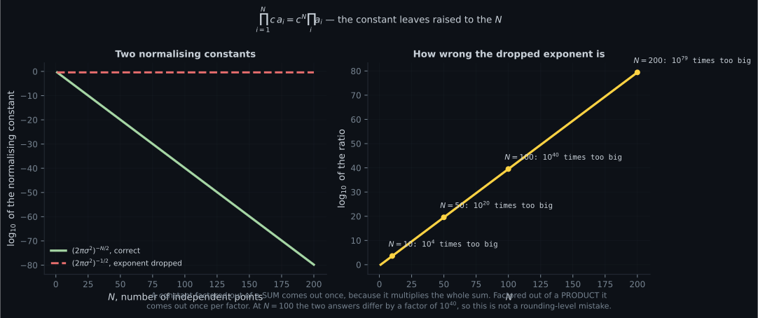
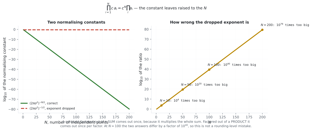
The constant comes out raised to the power , because it appeared in every one of the factors. This exact step is why the Gaussian likelihood of independent points carries a out front (§6.5), and forgetting the exponent is a classic way to derive a wrong normalising constant.
Double sums
Section titled “Double sums”Two nested loops. The inner sum runs to completion for each value of the outer index. When the limits are constants — neither depends on the other index — you may swap them freely:
Both sides add up the same numbers; only the order changes, and addition does not care about order. Thinking of as a grid makes it obvious: one side sums the rows and then adds the row totals, the other sums the columns and adds the column totals.
Telescoping
Section titled “Telescoping”If the body is a difference of consecutive terms, almost everything cancels:
Write it out and every interior term appears once with a plus and once with a minus. What survives is the two endpoints. This is the discrete version of the Fundamental Theorem of Calculus, which the calculus refresher makes explicit, and it is the trick behind the monotone-improvement proof of EM in Chapter 11.
Worked example by hand
Section titled “Worked example by hand”Take with and , and check every rule against arithmetic.
| rule | expression | expansion | value |
|---|---|---|---|
| plain sum | |||
| Rule 1 | |||
| Rule 2 | |||
| Rule 3 | |||
| reindexed | |||
| product | |||
| product, Rule 1 | |||
| telescoping, |
The last row is worth pausing on. The body expands to , so the sum is — the sum of the first five odd numbers is . Telescoping gave the answer without adding anything.
Now the double sum. With over and :
| row total | |||
|---|---|---|---|
| column total |
Rows first: . Columns first: . Same answer, which is the swap rule made concrete. And note — when the body factorises as , the double sum factorises into a product of two single sums. That observation turns up whenever an expectation splits over independent variables (§6.4).
See it move
Section titled “See it move”Drag the limits. The highlighted cells are the terms the sum currently collects, and the running total is what a loop would accumulate.
Two things to notice. Moving the lower limit up removes terms from the front — the sum does not slide, it shrinks. And on the triangular setting the collected cells form a staircase, not a block: that is the shape the swap rule has to preserve, and it is why the limits change when you swap.
A sum runs over an index. A set is what you run over when there is no natural order.
The second is set-builder notation, and it reads left to right as: “the set of drawn from such that ”. The colon is “such that”; some authors use a vertical bar instead.
| notation | meaning |
|---|---|
| is an element of | |
| is not an element | |
| every element of is in | |
| union: in , or in , or both | |
| intersection: in both | |
| in but not in | |
| Cartesian product: all ordered pairs | |
| the empty set | |
| cardinality: how many elements |
Three of these do specific jobs later:
- is the definition of a subspace (§2.4): a subset that is itself a vector space.
- is how the orthogonal complement is characterised (§3.6), and how a feasible region is built from several constraints (§7.2).
- is why is written and why a joint distribution lives on a product space (§6.1).
The indicator function
Section titled “The indicator function”The bridge from a condition to arithmetic:
It lets a count be written as a sum. The number of correct predictions is
and dividing by gives accuracy. In NumPy the indicator is a boolean array and the sum is
(y_hat == y).sum(), because True behaves as . That equivalence is not a coincidence of the
language — it is the indicator function, implemented.
The zero-one loss of §8.2, the responsibilities of §11.3 and the hinge-loss counting argument of §12.2 are all indicator sums.
From scratch
Section titled “From scratch”import numpy as np
a = np.arange(1, 6) # a_i = i for i = 1..5
print("sum:", a.sum()) # 15
print("Rule 1 sum 3a_i == 3 sum a_i:", (3 * a).sum() == 3 * a.sum())
print("Rule 2 sum(a+b) == sum a + sum b:",
(a + 2).sum() == a.sum() + np.full(5, 2).sum())
print("Rule 3 sum of a constant:", np.full(5, 2).sum()) # 10
print("product:", a.prod()) # 120
print("Rule 1 for products, c^n:", (3 * a).prod(), "==", 3**5 * a.prod())
# Telescoping: sum of (i^2 - (i-1)^2) collapses to the endpoints.
b = np.arange(0, 6) ** 2 # b_0..b_5
print("telescoped:", np.diff(b).sum(), "== b_5 - b_0 =", b[-1] - b[0])
# Double sums: axis is the index you sum OVER.
A = np.outer(np.arange(1, 4), np.arange(1, 3)) # a_ij = i*j, 3x2
print("rows first:", A.sum(axis=1).sum(), " columns first:", A.sum(axis=0).sum())
print("factorises:", A.sum(), "==", np.arange(1, 4).sum() * np.arange(1, 3).sum())
# Triangular sum: the mask IS the inner limit j <= i.
i, j = np.indices((6, 6)) + 1
tri = np.where(j <= i, i * j, 0)
print("lower triangle:", tri.sum())
# The indicator function is a boolean array.
y = np.array([1, 0, 1, 1, 0])
y_hat = np.array([1, 0, 0, 1, 0])
print("correct:", (y_hat == y).sum(), "of", y.size,
" accuracy:", (y_hat == y).mean())
# Sets: unordered, no duplicates.
print({1, 1, 2} == {2, 1}, " but tuples keep order:", (1, 2) == (2, 1))sum: 15
Rule 1 sum 3a_i == 3 sum a_i: True
Rule 2 sum(a+b) == sum a + sum b: True
Rule 3 sum of a constant: 10
product: 120
Rule 1 for products, c^n: 29160 == 29160
telescoped: 25 == b_5 - b_0 = 25
rows first: 18 columns first: 18
factorises: 18 == 18
lower triangle: 266
correct: 4 of 5 accuracy: 0.8
True but tuples keep order: FalseOn real data
Section titled “On real data”Three claims made above are worth measuring rather than believing. Every number in these figures was computed, not estimated.
Reading the plot
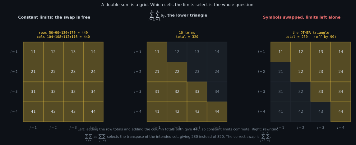
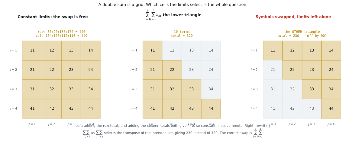
Section titled “Reading the plot”The first figure settles when you may swap. In the left panel the limits do not mention the other index, so both orders add up the same sixteen numbers and both reach — the row totals and the column totals are different decompositions of one number. In the middle panel the inner limit is , which selects ten cells totalling . The right panel is what happens if you write and stop there: it selects the ten cells of the upper triangle, totalling . The grid is deliberately asymmetric — , so while — because on a symmetric grid the two triangles would agree and this bug would be invisible in testing. Being out of wrong, or , is the kind of error that produces a plausible-looking but incorrect gradient.
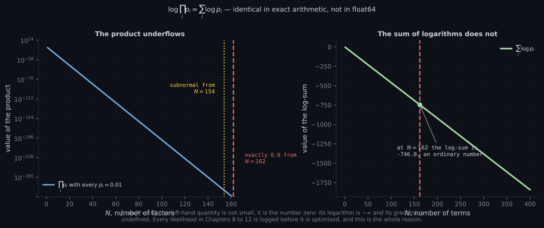
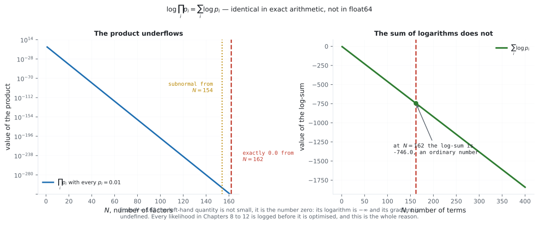
The second figure is the practical reason for logarithms. Reading the left panel: the product
stays representable for a while, drifts into the subnormal range at where it starts losing
precision silently, and reaches exactly 0.0 at . Not a small number — zero. Its
logarithm is , its gradient is undefined, and any optimiser handed it stops. The right panel
plots the same quantity as , which at is : an ordinary float with
plenty of room left. Nothing about the mathematics changed, only which of two algebraically identical
expressions was evaluated. A likelihood over even a small dataset has thousands of factors, which is
why you will not see an unlogged one anywhere in Chapters 8 to 12.
The third figure prices the exponent. The correct constant falls linearly on a log axis because each of the factors contributes; the version that pulls out just once is flat. The right panel is the ratio, and it grows without bound: at ten points, at a hundred, at two hundred. If you are optimising and this error is a constant with respect to , so the mean you recover is still right — which is precisely why the mistake survives. It is not constant with respect to , so the variance you recover is wrong, and nothing in the fit will tell you.
Pitfalls
Section titled “Pitfalls”Compare
Section titled “Compare”| you want to | sum | product |
|---|---|---|
| pull out a constant | comes out unchanged | comes out as |
| split over | yes, is linear | no |
| empty range | , the additive identity | , the multiplicative identity |
| turn into the other | of a sum is a product | of a product is a sum |
| NumPy | .sum(), np.add.reduce | .prod(), np.multiply.reduce |
| numerical risk | catastrophic cancellation | underflow or overflow |
The empty-range row is not trivia: an empty sum is and an empty product is , and both conventions make edge cases in recursive derivations work without a special case.
-
You need to pull the constant three out of a product of n terms. What comes out?
The constant appeared in every one of the n factors, so it comes out raised to the n. This is exactly the step that produces the normalising constant in an i.i.d. Gaussian likelihood.
pch.quizShowAnswer
B — Three to the power n — The constant appeared in every one of the n factors, so it comes out raised to the n. This is exactly the step that produces the normalising constant in an i.i.d. Gaussian likelihood.
-
A double sum has an inner limit that runs from one up to the outer index. Can you swap the two sums?
The same terms are being added either way, so a swap is possible, but the limits describe the region and must be rewritten to describe it column-wise instead of row-wise.
pch.quizShowAnswer
B — Yes, but the limits must be rewritten so they describe the same triangle — The same terms are being added either way, so a swap is possible, but the limits describe the region and must be rewritten to describe it column-wise instead of row-wise.
-
Why does machine learning almost always work with log likelihoods rather than likelihoods?
A product of many small probabilities underflows to zero; the sum of their logarithms does not. And because the logarithm is increasing, the maximum does not move — which is what makes the substitution legitimate.
pch.quizShowAnswer
B — A logarithm turns the product into a sum, which avoids floating-point underflow — A product of many small probabilities underflows to zero; the sum of their logarithms does not. And because the logarithm is increasing, the maximum does not move — which is what makes the substitution legitimate.
-
In NumPy, what does summing with axis equal to zero do to a two-dimensional array?
The axis names the index being eliminated. Collapsing the first index leaves one entry per column. Reading it as the index you sum away, rather than as a direction, removes the ambiguity that makes this error so common.
pch.quizShowAnswer
A — Collapses the first index, leaving one value per column — The axis names the index being eliminated. Collapsing the first index leaves one entry per column. Reading it as the index you sum away, rather than as a direction, removes the ambiguity that makes this error so common.
🧪 Try It Yourself
Section titled “🧪 Try It Yourself”Exercise 1 – A sum is a loop
Section titled “Exercise 1 – A sum is a loop”Exercise 2 – The constant comes out squared, cubed, …
Section titled “Exercise 2 – The constant comes out squared, cubed, …”Exercise 3 – Telescoping
Section titled “Exercise 3 – Telescoping”Exercise 4 – Swapping a triangular double sum
Section titled “Exercise 4 – Swapping a triangular double sum”Exercise 5 – An indicator sum is an accuracy
Section titled “Exercise 5 – An indicator sum is an accuracy”Recall card
Section titled “Recall card”- A sum is a loop with an accumulator — index, inclusive lower limit, inclusive upper limit, body.
- Sigma is linear: a constant factors out and sums split over addition, which is why gradients and expectations both pass straight through a sum.
- Pulling a constant out of a product raises it to the power n — the source of the exponent in an i.i.d. likelihood’s normalising constant.
- Log turns a product into a sum, which is the entire reason machine learning maximises log likelihoods.
- Double sums with constant limits swap freely; dependent limits swap only after rewriting them to describe the same region the other way round.
- Telescoping — a sum of consecutive differences collapses to the two endpoints, and it is the discrete Fundamental Theorem of Calculus.
- An empty sum is zero and an empty product is one, which is what makes recursive edge cases work without special-casing.
axisnames the index you sum away, not a direction — readaxis=0as eliminating the first index.- The indicator function turns a condition into arithmetic, and in NumPy it is just a boolean array being summed.
Next: what a function actually is, and the two properties Chapter 2 will demand of one — Functions, Limits, and Continuity.
pch.coffeeTagline
pch.coffeeCtapch.feedbackHeading
pch.feedbackSubheading