Vision Transformers (ViT)

Every page in this phase has used convolution: a small kernel slid over the image, weight-shared across positions, with locality built into the architecture. A vision transformer throws all of that away. Cut the image into patches, treat them as a set of tokens, and let attention decide which patch should look at which.

That sounds worse, and the usual summary is “ViTs need enormous datasets to beat convnets”. On the measurement here it is not what happened, so this page reports what the numbers said and explains the discrepancy rather than the folklore.

What you’ll learn

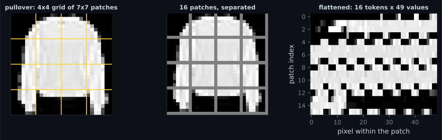
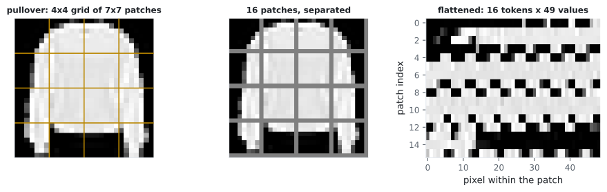
• Patching as a reshape: 28×28 → 16 tokens of 49 values, and it is lossless (max |rebuilt - original| = 0.00e+00).
• What a ViT has to buy that a convnet gets free: 1,024 parameters of position embedding, because a set has no order.
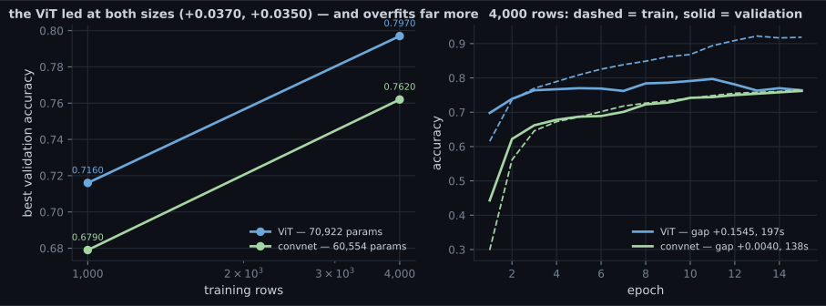
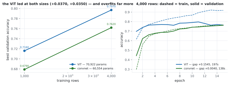
• The transformer block in Keras — LayerNormalization, MultiHeadAttention, residual, MLP — in about fifteen lines.
• The measured comparison: ViT 0.7970, convnet 0.7620 at 4,000 rows — with the ViT overfitting nearly four times as hard (train-val gap +0.1545 against +0.0040).
• Why token count, not image size, is the cost: attention entries grow with the square of the number of patches.
• What the attention heads actually did, including a head that mostly ignored position.

Patching is a reshape

28x28 into 16 tokens of 49 values

def patchify(images, patch=7):
    count, side = len(images), images.shape[1]
    grid = side // patch
    reshaped = images.reshape(count, grid, patch, grid, patch)
    return reshaped.transpose(0, 1, 3, 2, 4).reshape(count, grid * grid, patch * patch)

No information is lost — 28 × 28 = 784 = 16 × 49, and reversing the transpose reconstructs the image exactly. What is lost is adjacency: after the reshape, token 0 and token 1 are just two rows of a matrix, and nothing tells the model they were neighbours.

figure One image, three views: pixels, patches, tokens matplotlib

The right panel is what the transformer actually receives — a 16 by 49 matrix with no spatial structure at all. A convolution's kernel knows that pixel (3, 4) is next to (3, 5) because the architecture places them under the same kernel; the ViT has to learn that relationship from a position embedding and the data.

Component	Size	Parameters
patch projection (49 → 64)	one Dense	3,200
position embedding	16 × 64	1,024
one attention block (Q, K, V, out)	4 × (64×64 + 64)	16,640
one MLP block (64 → 128 → 64)	two Dense	16,576
Conv2D(64, 3) on 1 channel, for scale	—	640

The last row is the honest comparison for the input stage: a convolution buys its spatial prior for 640 parameters; the ViT spends 3,200 on projection and another 1,024 purely to reintroduce the notion of “where”. That is the inductive-bias trade, priced.

The block

A transformer block, pre-norm, with residuals

def block(x, width=64, heads=4):
    normed = keras.layers.LayerNormalization(epsilon=1e-6)(x)
    attention = keras.layers.MultiHeadAttention(num_heads=heads,
                                                key_dim=width // heads)(normed, normed)
    x = keras.layers.Add()([x, attention])              # residual
    normed = keras.layers.LayerNormalization(epsilon=1e-6)(x)
    hidden = keras.layers.Dense(width * 2, activation="gelu")(normed)
    hidden = keras.layers.Dense(width)(hidden)
    return keras.layers.Add()([x, hidden])              # residual

Three details are load-bearing, and each ties back to an earlier page:

• LayerNormalization, not BatchNormalization. Per-token statistics, no batch dependence, no moving averages to get wrong — the exact argument measured on Normalisation Beyond Batch.
• Pre-norm. Normalise before the sublayer and add the raw input back, so the residual path stays clean. Post-norm transformers need learning-rate warmup to train at all.
• Residuals in exactly the ResNet pattern — including the lesson from Famous CNN Architectures: the activation belongs inside the branch, never between the branch and the Add.

MultiHeadAttention(num_heads=4, key_dim=16) called as layer(normed, normed) is self-attention: queries, keys and values all come from the same tokens.

$$\mathrm{Attention}(Q, K, V) = \mathrm{softmax}\!\left(\frac{QK^\top}{\sqrt{d_k}}\right) V$$

Every token’s output is a weighted average of every token, with weights that depend on the content. Each query’s weights sum to 1 — Exercise 3 checks it — and with 16 tokens a head that ignored position entirely would put 0.0625 everywhere.

diagram Diagram mermaid

  flowchart TB
  A["28x28x1 image"] --> B["patchify: 16 tokens x 49"]
  B --> C["Dense 64
3,200 params"]
  C --> D["+ position embedding
1,024 params"]
  D --> E["block 1: LN -> MHA -> +
LN -> MLP -> +"]
  E --> F["block 2: same"]
  F --> G["LayerNorm"]
  G --> H["GlobalAveragePooling1D
over tokens"]
  H --> I["Dense 10 softmax"]

The measurement

Both models trained on Fashion-MNIST, 15 epochs, same seed, same optimiser:

Model	Rows	Parameters	Best val accuracy	Final train accuracy	Seconds
ViT	1,000	70,922	0.7160	0.8850	62.0
convnet	1,000	60,554	0.6790	0.7060	42.8
ViT	4,000	70,922	0.7970	0.9185	56.6
convnet	4,000	60,554	0.7620	0.7660	94.3

figure ViT against convnet at two dataset sizes matplotlib

The ViT led at both sizes, by 0.0370 and 0.0350 — the opposite of the usual claim, and the right panel shows why it is not a clean win: its train-val gap is +0.1545 against the convnet's +0.0040. The ViT is memorising and still generalising slightly better; the convnet has barely started to fit. Note also the timing inversion — the ViT was slower at 1,000 rows and faster at 4,000, because attention over 16 tokens parallelises where a convolution over 784 positions does not.

Why does this contradict the folklore? Because the folklore is about ImageNet-scale images, and none of its conditions hold here:

• 16 tokens. Attention over 16 patches is a tiny, well-conditioned problem. The data-hunger results come from 196 tokens (224×224 with 16×16 patches) and up, where the number of pairwise relationships to learn is 150× larger.
• A 7×7 patch is a quarter of the image. Each token already sees a large, meaningful region, so the model needs much less spatial reasoning than at 16×16 patches on a 224×224 photograph.
• Fashion-MNIST is centred and pose-normalised. The translation invariance a convolution provides for free is worth very little when every garment is already centred — the same reason augmentation hurt on this data.
• The convnet was not tuned to win. It is a plain three-block stack at 60,554 parameters against 70,922, and it stopped improving early.

The generalisable claim is not “ViTs beat convnets” but: a ViT’s advantage grows as the convolutional prior becomes less appropriate, and its cost grows as the square of the token count. On 28×28 centred greyscale with 16 tokens, the prior buys little and the cost is negligible.

Token count is the price

Image	Patch	Tokens	Attention entries	Relative to 16 tokens
28×28	7	16	256	1.0×
28×28	4	49	2,401	9.4×
64×64	8	64	4,096	16.0×
224×224	16	196	38,416	150.1×
224×224	8	784	614,656	2,401.0×

Self-attention compares every token with every other, so cost scales as $O(N^2)$ in the token count $N$ — and halving the patch size quadruples $N$, multiplying cost by 16. This single table explains most of the vision-transformer literature: windowed attention (Swin), pooling between stages, linear-attention approximations and convolutional stems all exist to keep $N$ small.

What the heads did

ViT test accuracy on the full split: 0.7640. Attention scores have shape (rows, heads, queries, keys) = (4, 4, 16, 16), and per-head spread — the gap between the most- and least-attended token, where 0.0625 would be perfectly uniform:

Row	True → predicted	Confidence	Head spreads
0	boot → boot	0.9885	0.2777, 0.1662, 0.1501, 0.2707
1	pullover → pullover	0.9570	0.6459, 0.3618, 0.3304, 0.1947
11	sandal → boot	0.9020	0.2056, 0.1905, 0.1565, 0.1792
12	sneaker → bag	0.6497	0.2021, 0.1643, 0.1472, 0.1966

figure Per-head attention for two correct and two incorrect predictions matplotlib

Head 0 on the pullover concentrates 0.648 of one query's attention on a single patch — a real, sharp preference. Most other heads sit between 0.15 and 0.29 against a uniform 0.0625, which is structured but diffuse. The two wrong rows are the useful ones: the sandal called 'boot' at confidence 0.9020 shows no attention pathology at all, which is the honest limit of attention maps as explanations — a confidently wrong model can look entirely normal.

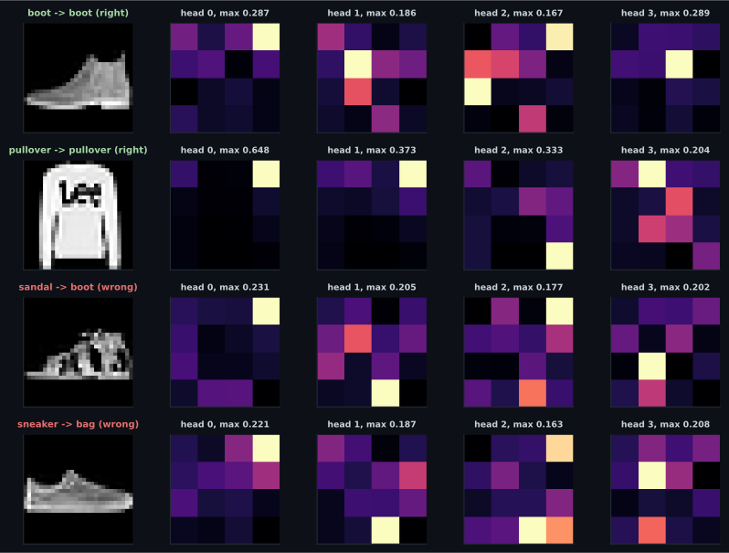
That last point deserves emphasis, because attention maps are widely published as explanations. The failure here is not visible in the attention. It has the same status as the Grad-CAM sanity check: a picture derived from a model is not automatically evidence about the model.

sketch Attention over 16 patches p5.js Pause Restart

Click a patch to make it the query. The weights are softmax over content similarity — drag the temperature to sharpen or flatten them, and watch the 0.0625 uniform line.

At temperature 1 the weights here sit near the uniform 0.0625, which is what the measured heads mostly did (maxima 0.16–0.29). Sharpen it and one patch takes almost everything — the behaviour of head 0 on the pullover, at 0.648.

sketch The measured table, ranked p5.js Pause Restart

Click a column to rank every row by it. The bars are that column's values and the highest and lowest are computed from the numbers, not written in.

Pitfalls

• Forgetting the position embedding. Attention is permutation-equivariant: without it the model literally cannot tell a shuffled image from the original.
• Using BatchNormalization in a transformer block. Per-token LayerNormalization is the whole reason the block trains without batch-statistics trouble.
• Post-norm without warmup. Add then normalise diverges at ordinary learning rates; pre-norm is the robust default.
• Shrinking the patch size to “see more detail”. Halving it quadruples the tokens and multiplies attention cost by 16 — measured 150× from 7×7 on 28×28 to 16×16 on 224×224.
• Quoting “ViTs need huge data” as a law. Measured here, a 70,922-parameter ViT beat a 60,554-parameter convnet at 1,000 rows. The claim is conditional on token count, patch scale and how well the convolutional prior fits the data.
• Ignoring the overfitting. The ViT’s +0.1545 train-val gap against +0.0040 is the real warning in that table: it wins while memorising, and it will need augmentation or regularisation long before the convnet does.
• Reading attention maps as explanations. A sandal was called a boot at 0.9020 confidence with entirely unremarkable attention.

Recap

• Patching is a lossless reshape: 28×28 → 16 tokens × 49 values, max |error| = 0.00e+00.
• Position must be bought: 1,024 parameters of embedding to replace what a convolution’s structure gives free.
• The block is pre-norm LayerNormalization → MultiHeadAttention → residual → MLP → residual, and each token’s output is a weighted average of all tokens.
• Measured on Fashion-MNIST: ViT 0.7160 / 0.7970 against convnet 0.6790 / 0.7620 at 1,000 / 4,000 rows — but with a train-val gap of +0.1545 against +0.0040.
• Attention cost is $O(N^2)$ in tokens: 256 entries at 16 tokens, 38,416 at 196, 614,656 at 784.
• Attention maps showed a sharp head (0.648 on one patch) and diffuse ones, and looked perfectly normal on a confidently wrong prediction.

Next

That closes Computer Vision. Sequences are next, and the first thing they break is the assumption that every input has the same size: Phase 4 — Sequence Models with RNNs.

pch.quizTag pch.quizDefaultTitle

1. Patching a 28x28 image into 16 tokens of 49 values loses no information (max error 0.00e+00). What does it lose?

   A Colour information B Adjacency — after the reshape nothing tells the model which patches were neighbours, which is why a position embedding has to be learned C Resolution, because the patches are downsampled D The channel dimension
   pch.quizShowAnswer

   B — Adjacency — after the reshape nothing tells the model which patches were neighbours, which is why a position embedding has to be learned — Self-attention is permutation-equivariant: shuffle the tokens and, without position embeddings, the output is the same.

2. The ViT beat the convnet at both dataset sizes here, contradicting the usual 'ViTs need huge data' claim. What is the most important reason?

   A The convnet was implemented incorrectly B This ViT has only 16 tokens and each patch covers a quarter of the image, so there is very little spatial reasoning left to learn — the data-hunger results come from 196 tokens and up C Fashion-MNIST is harder than ImageNet D Attention is inherently more parameter-efficient
   pch.quizShowAnswer

   B — This ViT has only 16 tokens and each patch covers a quarter of the image, so there is very little spatial reasoning left to learn — the data-hunger results come from 196 tokens and up — Fashion-MNIST is also centred and pose-normalised, so the translation invariance a convolution provides for free is worth very little here.

3. Why is halving the patch size expensive?

   A It doubles the number of parameters B It quadruples the token count, and attention compares every token with every other — so the cost grows by 16x C It requires more attention heads D It breaks the position embedding
   pch.quizShowAnswer

   B — It quadruples the token count, and attention compares every token with every other — so the cost grows by 16x — Measured: 256 attention entries at 16 tokens, 38,416 at 196, and 614,656 at 784. Swin's windowed attention and convolutional stems exist to keep that number small.

4. Why does a transformer block use LayerNormalization rather than BatchNormalization?

   A Because it is faster B Because it normalises each token using its own features — no batch dependence, no moving averages, and it behaves identically at batch size 1 C Because attention outputs are always positive D Because BatchNormalization does not support 3D tensors
   pch.quizShowAnswer

   B — Because it normalises each token using its own features — no batch dependence, no moving averages, and it behaves identically at batch size 1 — The same phase measured batch normalisation's moving-average lag breaking validation accuracy at short training runs; layer normalisation has no such state.

5. A sandal was classified as a boot with confidence 0.9020, and its attention maps looked unremarkable. What follows?

   A The attention scores were computed incorrectly B Attention maps are not automatically explanations — a confidently wrong model can have entirely normal-looking attention, the same caveat that applies to Grad-CAM C The model needs more heads D Sandals and boots are indistinguishable at 7x7 patches
   pch.quizShowAnswer

   B — Attention maps are not automatically explanations — a confidently wrong model can have entirely normal-looking attention, the same caveat that applies to Grad-CAM — Any picture derived from a model needs a control before it counts as evidence about the model.

🧪 Try It Yourself

pch.exerciseTag pch.exerciseTitle

pch.exerciseTag pch.exerciseTitle

pch.exerciseTag pch.exerciseTitle

pch.exerciseTag pch.exerciseTitle

pch.exerciseTag pch.exerciseTitle

pch.exerciseTag pch.exerciseTitle