Capstone 3 - A Generative Model You Can Defend

The first two capstones had an accuracy column. This one does not, and that single missing column changes everything about what the deliverable is.

Capstone 1 could be summarised in one number, 0.8773, and defended by pointing at a held-out split. Capstone 2 could be summarised in seven. A generative model produces images. There is no label to compare them against, no split that scores itself, and the only thing that feels like evidence — a grid of samples that look like digits — is the one thing you can produce without training anything at all.

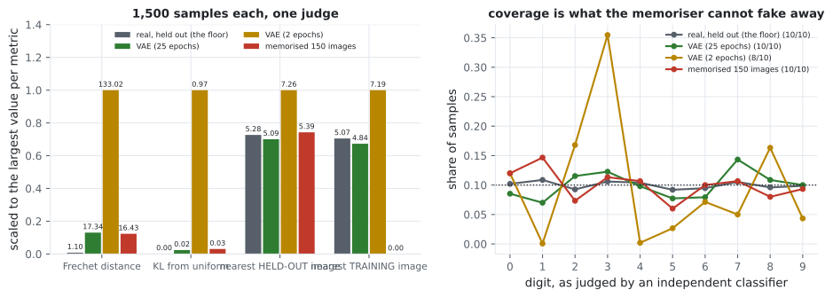
So the deliverable is not “a VAE”. It is a VAE and the evidence it works, and the evidence has to survive an adversary: a twelve-line program that generates nothing and copies 150 training images instead. On this page that adversary beats the real model on two of the four metrics.

What you’ll learn

• Why every generative metric needs a floor measured from real data, and what the floor is.
• The four numbers that make a generative result defensible, and what each one alone misses.
• How a memoriser defeats the obvious memorisation check — and which check catches it.
• How to tell whether the latent space actually supports sampling before you look at samples.

The setup

MNIST, 12,000 training images, a dense VAE with an 8-dimensional latent space, 25 epochs, 35 seconds on CPU. A separate classifier — trained on the same data, reaching 0.9477 validation accuracy — acts as the judge: it never sees the VAE, and it supplies both the feature space distances are measured in and the class predictions coverage is measured from.

Four sources get scored, 1,500 samples each:

Source	What it is
Real, held out	Real test digits, in neither reference set. The floor.
VAE, 25 epochs	The model the capstone is actually about.
VAE, 2 epochs	The same model trained badly. The control.
Memorised, 150 images	Copies of x_train[:150], tiled. The adversary.

The last two are the part people skip. Without the control you cannot show the metrics respond to quality at all; without the adversary you cannot show they respond to generation rather than to resemblance.

The report

figure 1,500 samples each, one judge matplotlib

The left panel is scaled per metric, so bar heights compare within a group and not across groups. The only column where the memoriser looks different from real data is the last one — distance to the nearest training image, 0.0035 against 5.0696. On the other three it is indistinguishable from a working model, and on Frechet distance it beats one.

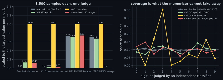
Source	Fréchet	Classes	KL from uniform	Judge confidence	Nearest held-out	Nearest training
Real, held out (floor)	1.101	10	0.0016	0.9690	5.2787	5.0696
VAE, 25 epochs	17.343	10	0.0234	0.8481	5.0886	4.8392
VAE, 2 epochs	133.022	8	0.9654	0.7833	7.2647	7.1922
Memorised, 150 images	16.425	10	0.0294	0.9952	5.3939	0.0035

Read the memoriser’s row before anything else. It scores 16.425 on Fréchet distance against the VAE’s 17.343 — better. It hits all ten classes. Its coverage KL is 0.0294 against the VAE’s 0.0234, effectively a tie. The judge is more confident about it than about real held-out data, 0.9952 against 0.9690, because it is looking at images it was trained on.

Three of the four metrics rank a program that generates nothing at or above the model that generates something. That is not a flaw in the metrics; it is what they measure. Fréchet distance asks whether the sample distribution matches the real one, and copies of real data trivially do.

The check that failed

The obvious defence is a nearest-neighbour check: for each generated image, find the closest real image and report the mean distance. If the model is copying, that distance collapses toward zero.

Here is what that check produced on the first attempt, comparing against held-out data:

Source	Distance to nearest held-out image
Real, held out	5.2787
VAE, 25 epochs	5.0886
Memorised, 150 images	5.3939

The memoriser scored higher than the VAE. The check did not merely fail to flag it — it ranked it as the least suspicious of the three.

The reason is a one-word bug in the experiment, not the code. The memoriser copies from x_train; the check measured against x_test. Copies of training images are perfectly ordinary digits as far as the test split is concerned — no closer to it than real held-out data is, which is exactly what 5.3939 against 5.2787 says.

The split you compare against is the experiment

A nearest-neighbour check against held-out data answers “is this sample a copy of some real image”. Only a check against the training data answers “is this a copy of something the model was shown”. They are different questions and the second is the one memorisation is about. Run the first and the report contains a column, a plausible number, and no information — the check looks like it ran.

Against the training set the same computation reads:

Source	Distance to nearest training image
Real, held out	5.0696
VAE, 25 epochs	4.8392
Memorised, 150 images	0.0035

0.0035 is floating-point noise on top of zero. The adversary is now unmissable, and the VAE’s 4.8392 sits just below the real-data floor of 5.0696 — slightly closer to the training set than real data is, which is what a model that has learned the distribution should look like.

The four numbers

Each metric catches something the others miss, which is why the report has four columns and not one.

Fréchet distance compares the mean and covariance of judge features between real and generated samples, treating each as a Gaussian:

$$d^2 = \lVert \mu_r - \mu_g \rVert^2 + \operatorname{tr}\!\left(\Sigma_r + \Sigma_g - 2\left(\Sigma_r \Sigma_g\right)^{1/2}\right)$$

It is a distribution-level measurement, so it is blind to whether individual samples are novel. It also has a floor that is not zero: two disjoint samples of real data score 1.101 here, not 0, because 1,500 samples estimate $\mu$ and $\Sigma$ imperfectly. Quoting 17.343 without that floor is quoting a number with no scale.

Coverage runs the judge over the samples and measures how far the predicted class histogram is from uniform:

$$D_{\mathrm{KL}}(u \parallel p) = \sum_{k=1}^{K} u_k \log \frac{u_k}{p_k}, \qquad u_k = \frac{1}{K}$$

This is the mode-collapse detector, and it is the one metric where the 2-epoch control fails loudly: 0.9654 against the trained model’s 0.0234, with only 8 of 10 classes produced at all.

Judge confidence is the mean maximum softmax probability — how typical the samples look. Note that it moves the wrong way for the memoriser (0.9952, above real data’s 0.9690), which is itself a signal: samples the judge finds easier than real data are usually samples the judge has memorised too.

Nearest-training distance is the novelty check, and per the section above it only works against the split the model trained on.

diagram Diagram mermaid

  flowchart TD
  S["1,500 samples"] --> F["Frechet distance
vs the real floor"]
  S --> C["coverage KL
+ classes hit"]
  S --> N["nearest TRAINING image"]
  S --> G["uncurated grid"]
  F --> V{"defensible?"}
  C --> V
  N --> V
  G --> V
  V -->|"any one alone"| W["no - the memoriser
passes three of four"]
  V -->|"all four + a control"| Y["yes"]

Does the latent space support sampling?

Everything above scores samples. This checks something earlier: whether drawing $z \sim \mathcal{N}(0, I)$ and decoding is even a meaningful operation.

figure Encoder means for the held-out set, 8 latent dimensions matplotlib

The right panel is the check that matters. Encoder means sit at mean radius 3.1233 from the origin; samples from the prior sit at 2.7348. Those distributions overlap heavily, so a vector drawn from the prior lands in a region the decoder has actually seen. If the encoder radius were far from the prior's, every sample would be decoded from a place the model never visited during training.

Two things get measured:

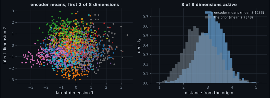
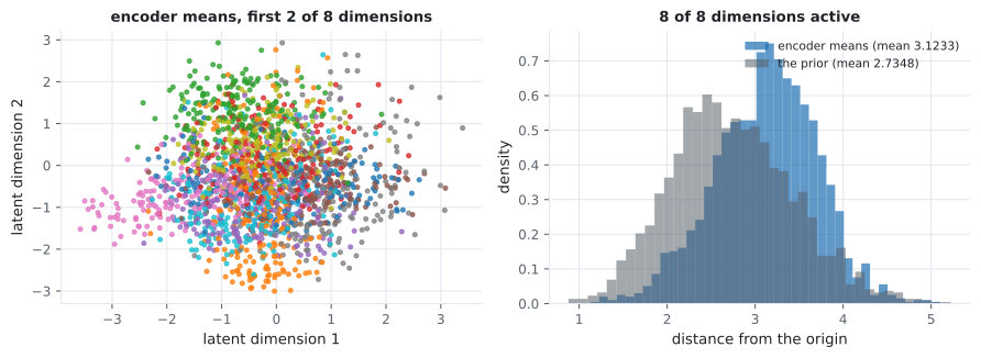
Active dimensions. A VAE can satisfy its KL term by switching latent dimensions off — driving the posterior for a dimension to exactly the prior, which costs zero KL and carries zero information. Here 8 of 8 dimensions have a standard deviation above 0.1 across the test set:

text

1.049  1.070  1.115  1.141  1.256  0.948  1.166  1.056

None collapsed. An 8-dimensional latent space that is really a 3-dimensional one still produces images, and the sample grid will not tell you.

Radius agreement. In $d$ dimensions a standard normal concentrates on a shell of radius approximately $\sqrt{d}$, not near the origin — for $d = 8$ that is 2.7348, measured. The encoder means average 3.1233. Close enough that the prior samples where the decoder was trained; a posterior sitting at, say, 0.9 would mean prior sampling was extrapolation dressed up as generation.

The uncurated grid

figure The first 36 samples from each source, nothing selected matplotlib

Left to right: the trained VAE, the undertrained control, the memoriser. The memoriser's grid is the sharpest of the three by a wide margin — which is the whole problem with sample grids as evidence. The control's grid, by contrast, is honestly bad, and that is what the metrics are calibrated to detect.

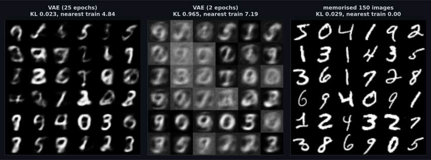
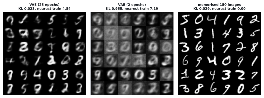
Sample grids belong in the report, but with two rules. Uncurated — the first $n$ samples from a fixed seed, not the best $n$. And beside the control, because a grid alone has no scale: the memoriser’s grid is the most convincing one on this page.

sketch Which check catches which failure p5.js Pause Restart

Click a generator to score it. Each metric lights up green when it would pass and red when it would catch that generator - no single row catches everything.

What to hand in

1. The floor, measured on real data at the same sample count as everything else. 1.101 here. Without it, 17.343 is a number with no units.
2. An undertrained control — the same model, trained badly. 2 epochs: Fréchet 133.022, 8 of 10 classes, KL 0.9654. It costs one extra run and it is the only thing that shows the metrics respond to quality rather than to noise.
3. A memorisation adversary, and the check that catches it, against the training split. Report the number, not the reassurance.
4. All four metrics, including the ones your model loses on. The VAE loses to the memoriser on Fréchet distance. Say so, and say why the result still stands.
5. The latent diagnostics: active dimensions (8 of 8) and encoder radius against prior radius (3.1233 against 2.7348), which justify prior sampling before any sample is shown.
6. An uncurated grid from a fixed seed, next to the control’s grid.

sketch The measured table, ranked p5.js Pause Restart

Click a column to rank every row by it. The bars are that column's values and the highest and lowest are computed from the numbers, not written in.

Pitfalls

• Reporting Fréchet distance without a floor. Two samples of real data score 1.101 at $n = 1{,}500$; the floor moves with $n$, so it has to be measured at the same $n$.
• Running the memorisation check against the wrong split. 5.3939 against held-out data, 0.0035 against training data — same code, same adversary, opposite conclusions.
• Curating the sample grid. The memoriser’s grid is the best-looking one on this page.
• Treating high judge confidence as quality. The memoriser scored 0.9952, above real data.
• Skipping the control. Metrics that never saw a bad model have not been shown to detect one.
• Assuming all latent dimensions are used. A collapsed dimension costs zero KL and carries zero information, and nothing in the sample grid reveals it.
• Comparing scores across judges or feature spaces. Fréchet distance is only comparable against numbers computed with the same feature extractor on the same number of samples.

Recap

• A generative result has no accuracy column, so the deliverable is the evaluation, not the model.
• A memoriser copying 150 training images beat the VAE on Fréchet distance (16.425 against 17.343), tied it on coverage, and scored higher judge confidence than real data.
• The nearest-neighbour check against held-out data ranked the memoriser as the least suspicious source, at 5.3939. Against training data it read 0.0035.
• The floor is not zero: real against real scored 1.101 at 1,500 samples.
• The undertrained control failed loudly — 133.022, 8 of 10 classes, KL 0.9654 — which is what makes the trained model’s numbers mean something.
• All 8 latent dimensions stayed active, and the encoder radius of 3.1233 sits close enough to the prior’s 2.7348 that prior sampling is defensible.

Next

That is the module. Nine phases, from a perceptron fitted by hand to a generative model with an evaluation that survives an adversary. Back to the Deep Learning overview.

pch.quizTag pch.quizDefaultTitle

1. A program that copies 150 training images scored 16.425 on Fréchet distance while the trained VAE scored 17.343. What does that show?

   A The memoriser is a better generative model B Fréchet distance is broken and should not be used C Fréchet distance measures distribution match, which copied real data trivially achieves - so it cannot detect memorisation on its own D The VAE needs more epochs
   pch.quizShowAnswer

   C — Fréchet distance measures distribution match, which copied real data trivially achieves - so it cannot detect memorisation on its own

2. The nearest-neighbour check gave the memoriser 5.3939 against held-out data and 0.0035 against training data. Why the difference?

   A The test split is noisier than the training split B The memoriser copies from the training split, so its samples are ordinary unseen digits relative to the test split and exact matches relative to the training split C The distance metric is unstable at small sample sizes D Held-out images have different pixel scaling
   pch.quizShowAnswer

   B — The memoriser copies from the training split, so its samples are ordinary unseen digits relative to the test split and exact matches relative to the training split

3. Two disjoint samples of real held-out data scored 1.101 on Fréchet distance rather than 0. What is that number?

   A A bug in the implementation B Evidence that the test set is not representative C The estimation floor - 1,500 samples estimate the mean and covariance imperfectly, so any generative score must be read against it D The irreducible error of the judge classifier
   pch.quizShowAnswer

   C — The estimation floor - 1,500 samples estimate the mean and covariance imperfectly, so any generative score must be read against it

4. Why is an undertrained control (the same VAE at 2 epochs) part of the deliverable?

   A To show the model improves with training B To demonstrate that the metrics respond to quality - without a known-bad source, nothing shows the metrics can detect one C To provide a second set of samples for the grid D To measure how long training takes
   pch.quizShowAnswer

   B — To demonstrate that the metrics respond to quality - without a known-bad source, nothing shows the metrics can detect one

5. All 8 latent dimensions had standard deviation above 0.1, and encoder means averaged 3.1233 from the origin against the prior's 2.7348. What do those two facts establish?

   A That the VAE reconstructs its inputs accurately B That the samples will be sharp C That no dimension collapsed to the prior, and that vectors drawn from the prior land where the decoder was actually trained - so prior sampling is meaningful D That the latent space is 8-dimensional
   pch.quizShowAnswer

   C — That no dimension collapsed to the prior, and that vectors drawn from the prior land where the decoder was actually trained - so prior sampling is meaningful

6. The judge classifier was more confident about the memoriser's images (0.9952) than about real held-out data (0.9690). What should that be read as?

   A Evidence the memoriser produces high-quality images B A signal - samples the judge finds easier than real data are typically samples it was trained on C A miscalibration of the judge that invalidates the report D Proof the judge overfitted the test set
   pch.quizShowAnswer

   B — A signal - samples the judge finds easier than real data are typically samples it was trained on

🧪 Try It Yourself

pch.exerciseTag pch.exerciseTitle

pch.exerciseTag pch.exerciseTitle

pch.exerciseTag pch.exerciseTitle

pch.exerciseTag pch.exerciseTitle

pch.exerciseTag pch.exerciseTitle

pch.exerciseTag pch.exerciseTitle