Optimization Using Gradient Descent

Every training loop in the second half of this book is a variation on one line:

$$\mathbf{x}_{i+1} = \mathbf{x}_i - \gamma_i\big((\nabla f)(\mathbf{x}_i)\big)^\top$$

That is it. Chapter 5 built the $\nabla f$; this page is about the $\gamma_i$, and about what the line can and cannot promise. The short version: it always goes downhill, it never tells you which valley you are in, and there are two ways to choose $\gamma$ badly for every one way to choose it well.

What you’ll learn

• Why setting the derivative to zero is the definition of a stationary point but almost never a usable method (§7.1, and the Abel–Ruffini theorem).
• Equation 7.6, the gradient descent update, and why it carries a transpose.
• Example 7.1 reproduced to the digit — including why the book’s $\mathbf{x}_1 = [-1.98, 1.21]^\top$ is exactly right.
• The step-size ceiling $\gamma < 2/L$ and the fastest step size $2/(\mu + L)$, both measured against a sweep of 136 values.
• Why a step size a hair past the ceiling can look like it is working for 30,000 iterations before it visibly fails.
• The condition number $\kappa = \sigma_{\max}/\sigma_{\min}$ (§4.5), and why it — not the step size — is the thing that makes gradient descent hopeless.
• That the famous “zigzag” is a transient: successive steps start almost reversed and end almost parallel.

Intuition: a ball, a hill, and no map

You are somewhere on a landscape in fog. You can feel the slope under your feet — that is the gradient — and nothing else. You cannot see the horizon, you do not know how many valleys there are, and you have no idea how far away the bottom is.

Two decisions follow, and they are the whole of this page:

• Which way? Downhill. The gradient points uphill (§5.2), so you go the other way. This decision is free and always correct.
• How far? Nobody tells you. Step too short and you are still walking at sunset. Step too long and you cross the valley and land higher up than you started.

The first decision is a one-liner. The second is a research field.

diagram What gradient descent needs, and what it cannot supply mermaid

  flowchart TD
  F["objective f, differentiable
Chapter 5"] --> G["gradient at the current point
Eq 5.40"]
  G --> D["descent direction
the negative gradient"]
  D --> U["update, Eq 7.6
x - gamma * grad"]
  S["step size gamma
Section 7.1.1"] --> U
  U --> U
  U --> R["a LOCAL minimum"]
  C["curvature: mu and L
the Hessian, Eq 5.147"] -.->|"caps gamma at 2/L"| S
  C -.->|"kappa = L/mu sets the speed"| R
  X["which valley?"] -.->|"decided by x0 alone"| R
  style X stroke-dasharray: 4 3
  style C stroke-dasharray: 4 3

The two dashed inputs are the honest part of the diagram. Curvature governs both the largest step you may take and how fast you converge, but the algorithm never looks at it. And the starting point alone decides which minimum you end up in, with nothing in the gradient to warn you.

The math

The problem

$$\min_{\mathbf{x}} f(\mathbf{x})$$

for a differentiable $f : \mathbb{R}^d \to \mathbb{R}$. By convention, machine learning minimises — if you have something to maximise, negate it. The book is explicit that this chapter assumes differentiability so that a gradient exists everywhere; §7.4 points at subgradient methods for when that fails.

Why not just set the derivative to zero?

Because you usually cannot solve the resulting equation. Take the book’s opening example:

$$\ell(x) = x^4 + 7x^3 + 5x^2 - 17x + 3$$ $$\frac{\mathrm{d}\ell(x)}{\mathrm{d}x} = 4x^3 + 21x^2 + 10x - 17$$

This is a cubic, so it has three real roots here and they are findable. Go one degree higher and you are stuck: by the Abel–Ruffini theorem there is no general algebraic solution for polynomials of degree five or more. And a neural network’s stationarity condition is not a polynomial at all.

So: stationary points are the definition of where an optimum can be, and root-finding is not a general method for locating them. That gap is why the rest of the chapter exists.

Classifying what you find

$$\frac{\mathrm{d}^2\ell(x)}{\mathrm{d}x^2} = 12x^2 + 42x + 10$$

Positive at a stationary point means a minimum, negative means a maximum. Solving $\ell'(x) = 0$ exactly rather than reading the plot gives

$x$	$\ell(x)$	$\ell''(x)$	verdict
$-4.480268$	$-47.074790$	$+62.7024$	global minimum
$-1.432112$	$+21.246724$	$-25.5374$	maximum
$+0.662381$	$-3.839903$	$+43.0850$	local minimum

The book quotes the visual estimates $-4.5$, $-1.4$, $0.7$ and a minimum value of “approximately $-47$”. Those are good reads: the exact values are $-4.4803$, $-1.4321$, $0.6624$ and $-47.0748$.

The update

Gradient descent is a first-order method: it uses $f$ and $\nabla f$, nothing else. Starting from $\mathbf{x}_0$,

$$\mathbf{x}_1 = \mathbf{x}_0 - \gamma\big((\nabla f)(\mathbf{x}_0)\big)^\top$$

and in general

$$\mathbf{x}_{i+1} = \mathbf{x}_i - \gamma_i\big((\nabla f)(\mathbf{x}_i)\big)^\top$$

Why the transpose. This module follows the book’s convention that a gradient is a row vector (§5.2, Equation 5.40). $\mathbf{x}_i$ is a column. You cannot subtract a $1 \times d$ row from a $d \times 1$ column, so the gradient is transposed back into a column first. It is a bookkeeping detail with no mathematical content, and it is exactly the kind of thing the typeface convention of §0.2 exists to catch.

For a small enough $\gamma \geq 0$ we get $f(\mathbf{x}_1) \leq f(\mathbf{x}_0)$, and the sequence $f(\mathbf{x}_0) \geq f(\mathbf{x}_1) \geq \dots$ converges to a local minimum. Note what is not claimed: not the global minimum, and not quickly.

Contour lines

A useful second picture. The set where $f(\mathbf{x}) = c$ is a contour line, and the gradient is everywhere orthogonal to it. So the descent direction always crosses the contours at right angles. On a circular bowl that points straight at the centre. On a long thin valley it points at the near wall, not at the bottom — which is the entire reason gradient descent zigzags, and the subject of the next page.

Worked example by hand

This is the book’s Example 7.1, done in full. The objective is a quadratic in two variables:

$$f\!\begin{bmatrix}x_1\\x_2\end{bmatrix} = \frac{1}{2}\begin{bmatrix}x_1\\x_2\end{bmatrix}^\top\begin{bmatrix}2&1\\1&20\end{bmatrix}\begin{bmatrix}x_1\\x_2\end{bmatrix} - \begin{bmatrix}5\\3\end{bmatrix}^\top\begin{bmatrix}x_1\\x_2\end{bmatrix}$$

with gradient

$$\nabla f\!\begin{bmatrix}x_1\\x_2\end{bmatrix} = \begin{bmatrix}x_1\\x_2\end{bmatrix}^\top\begin{bmatrix}2&1\\1&20\end{bmatrix} - \begin{bmatrix}5\\3\end{bmatrix}^\top$$

Write $\mathbf{A}$ for the matrix and $\mathbf{b}$ for the vector, so $f(\mathbf{x}) = \tfrac{1}{2}\mathbf{x}^\top\mathbf{A}\mathbf{x} - \mathbf{b}^\top\mathbf{x}$ and, transposed into a column, $\nabla f(\mathbf{x})^\top = \mathbf{A}\mathbf{x} - \mathbf{b}$.

Step 0. Start at $\mathbf{x}_0 = [-3, -1]^\top$ with $\gamma = 0.085$.

$$\mathbf{A}\mathbf{x}_0 = \begin{bmatrix}2&1\\1&20\end{bmatrix}\begin{bmatrix}-3\\-1\end{bmatrix} = \begin{bmatrix}-6-1\\-3-20\end{bmatrix} = \begin{bmatrix}-7\\-23\end{bmatrix}$$ $$\nabla f(\mathbf{x}_0)^\top = \begin{bmatrix}-7\\-23\end{bmatrix} - \begin{bmatrix}5\\3\end{bmatrix} = \begin{bmatrix}-12\\-26\end{bmatrix}$$

Both components are negative, so the negative gradient points north and east — exactly as the book says.

Step 1.

$$\mathbf{x}_1 = \begin{bmatrix}-3\\-1\end{bmatrix} - 0.085\begin{bmatrix}-12\\-26\end{bmatrix} = \begin{bmatrix}-3 + 1.02\\-1 + 2.21\end{bmatrix} = \begin{bmatrix}-1.98\\1.21\end{bmatrix}$$

Matching the book exactly, and note it is exact rather than rounded: $0.085 \times 12 = 1.02$ and $0.085 \times 26 = 2.21$.

Step 2. Repeat at $\mathbf{x}_1$:

$$\mathbf{A}\mathbf{x}_1 = \begin{bmatrix}-3.96+1.21\\-1.98+24.20\end{bmatrix} = \begin{bmatrix}-2.75\\22.22\end{bmatrix}, \qquad \nabla f(\mathbf{x}_1)^\top = \begin{bmatrix}-7.75\\19.22\end{bmatrix}$$ $$\mathbf{x}_2 = \begin{bmatrix}-1.98\\1.21\end{bmatrix} - 0.085\begin{bmatrix}-7.75\\19.22\end{bmatrix} = \begin{bmatrix}-1.321250\\-0.423700\end{bmatrix}$$

which rounds to the book’s $[-1.32, -0.42]^\top$. Notice that $x_2$ has swung from $+1.21$ to $-0.42$ in a single step: the iterate crossed the valley. That is the zigzag, visible after two steps.

Where it is going. This particular objective can be solved exactly, by setting the gradient to zero:

$$\mathbf{A}\mathbf{x}^* = \mathbf{b} \quad\Longrightarrow\quad \mathbf{x}^* = \mathbf{A}^{-1}\mathbf{b} = \frac{1}{39}\begin{bmatrix}20&-1\\-1&2\end{bmatrix}\begin{bmatrix}5\\3\end{bmatrix} = \frac{1}{39}\begin{bmatrix}97\\1\end{bmatrix}$$

using $\det\mathbf{A} = 40 - 1 = 39$. So $\mathbf{x}^* = [2.487179, 0.025641]^\top$ and $f(\mathbf{x}^*) = -6.256410$. After three gradient steps we are at $f = 5.576$, still more than $11$ above the answer.

The two numbers that decide the speed. The eigenvalues of $\mathbf{A}$ satisfy $\lambda^2 - 22\lambda + 39 = 0$, so

$$\lambda = \frac{22 \pm \sqrt{484 - 156}}{2} = \frac{22 \pm \sqrt{328}}{2}$$

giving $\mu = 1.944615$ and $L = 20.055385$, hence $\kappa = L/\mu = 10.313294$. Everything on the rest of this page is a consequence of those two numbers.

See it move

Start with the book’s own configuration. The trajectory below is Example 7.1, and the frames step through the same arithmetic you just did by hand.

optExample 7.1, one step at a timegradient descent

theta (2.4, 1.8)loss 9|grad| 6steps 0

1theta = theta_02for t in range(steps):3    g = grad_f(theta)4    theta = theta - lr * g          # downhill, scaled by lr

loss9|grad|6lr0.25

startStarting at (2.4, 1.8) on a well-conditioned bowl, f(x, y) = x² + y². The Hessian is 2I, so every direction curves the same amount and the gradient points straight at the minimum. The loss is 9 and the gradient is (4.8, 3.6) — the direction of steepest ASCENT, so every method below goes the other way.

Play‹›1/25⟲

Frames 1 to 3 are the hand calculation above. Watch the second component swing from positive to negative: that is the iterate crossing the valley, and it is what the condition number of 10.3 buys you.

Now the pathological case. Same algorithm, same step-size rule, a surface whose curvature ratio is far worse:

optThe same method on a ravinegradient descent

theta (-8.5, 1.6)loss 16.413|grad| 16.02steps 0

1theta = theta_02for t in range(steps):3    g = grad_f(theta)4    theta = theta - lr * g          # downhill, scaled by lr

loss16.413|grad|16.02lr0.16

startStarting at (-8.5, 1.6) on a ravine, f(x, y) = 0.05x² + 5y². The Hessian is diag(0.1, 10), so κ = 100: the surface curves a hundred times more steeply across the valley than along it. The loss is 16.413 and the gradient is (-0.85, 16) — the direction of steepest ASCENT, so every method below goes the other way.

Play‹›1/25⟲

The gradient is nearly orthogonal to the direction of the minimum for almost the whole run, so the iterates hop between the walls and creep along the floor. Nothing is wrong with the step size; the geometry is the problem.

And the case that gradient descent cannot detect at all:

optA stationary point that is not a minimumgradient descent

theta (2.2, 0.08)loss 4.834|grad| 4.4steps 0

1theta = theta_02for t in range(steps):3    g = grad_f(theta)4    theta = theta - lr * g          # downhill, scaled by lr

loss4.834|grad|4.4lr0.16

startStarting at (2.2, 0.08) on a saddle, f(x, y) = x² − y². The gradient vanishes at the origin but it is not a minimum: the Hessian has one positive and one negative eigenvalue. The loss is 4.834 and the gradient is (4.4, -0.16) — the direction of steepest ASCENT, so every method below goes the other way.

Play‹›1/25⟲

The gradient vanishes at the origin, so the update stalls there even though the point is a maximum in one direction. First-order information cannot distinguish this from a minimum — that takes the Hessian, from Section 5.7.

The step-size question deserves a sketch of its own. Below, the ceiling is a real number you can walk up to:

sketch Walk the step size up to the ceiling and over it p5.js Pause Restart

Drag the step-size knob. The sketch runs gradient descent on Example 7.1's quadratic from the book's starting point and draws the path over the contours. The ceiling 2/L is marked on the knob track; the interesting part is what happens just below and just above it.

From scratch

Twenty lines of NumPy, no optimiser library, reproducing every number claimed above.

gradient_descent.py

import numpy as np
 
# Example 7.1's quadratic: f(x) = 1/2 x^T A x - b^T x
A = np.array([[2.0, 1.0], [1.0, 20.0]])
b = np.array([5.0, 3.0])
 
def f(x):
    return 0.5 * x @ A @ x - b @ x
 
def grad(x):
    # Equation 7.8. The book writes the gradient as a ROW; NumPy hands back a
    # flat array, which we treat as the column that Equation 7.6 subtracts.
    return A @ x - b
 
def descend(x0, gamma, steps):
    x = np.asarray(x0, dtype=float)
    path = [x.copy()]
    for _ in range(steps):
        x = x - gamma * grad(x)
        path.append(x.copy())
    return np.array(path)
 
# --- the book's own iterates, Example 7.1 -----------------------------------
path = descend([-3.0, -1.0], gamma=0.085, steps=3)
for i, x in enumerate(path):
    print(f"x{i} = [{x[0]:+.4f}, {x[1]:+.4f}]   f = {f(x):+.6f}")
 
# --- where it is heading ----------------------------------------------------
xstar = np.linalg.solve(A, b)          # setting the gradient to zero
print(f"\nx* = [{xstar[0]:.6f}, {xstar[1]:.6f}]   f(x*) = {f(xstar):.6f}")
print("gradient at x* is zero:", np.allclose(grad(xstar), 0))
 
# --- the two numbers that govern everything --------------------------------
mu, L = np.linalg.eigvalsh(A)
print(f"\nmu = {mu:.6f}   L = {L:.6f}   kappa = {L / mu:.6f}")
print(f"divergence threshold  2/L      = {2 / L:.6f}")
print(f"fastest step size     2/(mu+L) = {2 / (mu + L):.6f}")
 
# --- so does the step size actually matter? --------------------------------
def steps_to_tolerance(gamma, tol=1e-8, cap=200_000):
    x = np.array([-3.0, -1.0])
    for k in range(cap):
        if np.linalg.norm(x - xstar) < tol:
            return k
        x = x - gamma * grad(x)
        if not np.all(np.isfinite(x)) or np.linalg.norm(x) > 1e12:
            return -1
    return cap
 
print("\n gamma      steps to 1e-8")
for gamma in (0.0100, 0.0850, 0.0909, 0.0990, 0.0997, 0.0998, 0.1050):
    k = steps_to_tolerance(gamma)
    print(f" {gamma:.4f}   {'diverged' if k < 0 else k}")

text

x0 = [-3.0000, -1.0000]   f = +40.000000
x1 = [-1.9800, +1.2100]   f = +22.435600
x2 = [-1.3213, -0.4237]   f = +11.978082
x3 = [-0.6356, +0.6639]   f = +5.576037
 
x* = [2.487179, 0.025641]   f(x*) = -6.256410
gradient at x* is zero: True
 
mu = 1.944615   L = 20.055385   kappa = 10.313294
divergence threshold  2/L      = 0.099724
fastest step size     2/(mu+L) = 0.090909
 
 gamma      steps to 1e-8
 0.0100   1025
 0.0850   112
 0.0909   104
 0.0990   1280
 0.0997   39113
 0.0998   diverged
 0.1050   diverged

Read the last block carefully, because it is the point of the page. Going from $\gamma = 0.0909$ to $\gamma = 0.0997$ — a $9.7\%$ increase — makes the method 376 times slower. One more nudge and it does not converge at all.

§7.1.1 Step-size

The book’s framing: the step size, also called the learning rate, is a genuine design choice, and both failure modes are real.

• Too small: every step is a descent step, so nothing goes wrong. It is simply slow, and “slow” here can mean thousands of iterations for a two-variable problem.
• Too large: gradient descent overshoots, fails to converge, or diverges outright.

For the quadratic $f(\mathbf{x}) = \tfrac12\mathbf{x}^\top\mathbf{A}\mathbf{x} - \mathbf{b}^\top\mathbf{x}$ the threshold is exact and worth knowing. Along the eigendirection with eigenvalue $\lambda$, one step multiplies the error by $|1 - \gamma\lambda|$. Every mode must contract, so we need $|1 - \gamma\lambda| < 1$ for all $\lambda$, which gives

$$0 < \gamma < \frac{2}{L}, \qquad L = \lambda_{\max}$$

and the choice that makes the worst mode contract fastest balances the extremes:

$$\gamma^{\star} = \frac{2}{\mu + L}, \qquad \text{giving a rate of } \frac{\kappa - 1}{\kappa + 1}$$

For Example 7.1 that is $2/22 = 0.090909$ with a rate of $0.823217$. The measured best over $136$ sampled step sizes is $104$ iterations, at exactly that value.

Adaptive step sizes

Rather than guessing, rescale $\gamma$ as you go. The book gives two heuristics (Toussaint, 2012):

1. If the function value increased after a step, the step was too large. Undo the step and decrease $\gamma$.
2. If the function value decreased, the step could have been bigger. Increase $\gamma$.

Why the “undo” is not wasted work

Throwing away a computed step looks wasteful. It buys something specific: monotonic convergence. With the undo in place, $f$ never increases, so the run cannot wander off and you can use “did $f$ go up?” as a correctness check. Without it, a single overlarge step can move you to a worse region that takes hundreds of steps to escape. Cheap insurance against an expensive failure.

Example 7.2: solving a linear system by descent

Given $\mathbf{A}\mathbf{x} = \mathbf{b}$, minimise the squared error

$$\lVert\mathbf{A}\mathbf{x} - \mathbf{b}\rVert^2 = (\mathbf{A}\mathbf{x} - \mathbf{b})^\top(\mathbf{A}\mathbf{x} - \mathbf{b})$$

whose gradient with respect to $\mathbf{x}$ is

$$\nabla_{\mathbf{x}} = 2(\mathbf{A}\mathbf{x} - \mathbf{b})^\top\mathbf{A}$$

Feed that straight into Equation 7.6 and you have an iterative linear solver. For this particular problem you should not: setting the gradient to zero gives the normal equations, which lstsq solves exactly in one call. Chapter 9 develops that properly. The example is here because it is the smallest honest instance of the pattern, and because it exposes the real bottleneck.

The condition number is the bottleneck

$$\kappa = \frac{\sigma(\mathbf{A})_{\max}}{\sigma(\mathbf{A})_{\min}}$$

the ratio of largest to smallest singular value (§4.5). The book’s reading of it is the one to keep: $\kappa$ measures the ratio of the most curved direction to the least curved one. A large $\kappa$ is a long thin valley — steep across, nearly flat along.

The fix is preconditioning: instead of $\mathbf{A}\mathbf{x} - \mathbf{b} = \mathbf{0}$, solve

$$\mathbf{P}^{-1}(\mathbf{A}\mathbf{x} - \mathbf{b}) = \mathbf{0}$$

choosing $\mathbf{P}$ so that $\mathbf{P}^{-1}\mathbf{A}$ has a better condition number while $\mathbf{P}^{-1}$ stays cheap to apply. Those two goals pull against each other — $\mathbf{P} = \mathbf{A}$ gives $\kappa = 1$ and is exactly as hard as the original problem — and navigating that trade-off is its own literature.

On real data

figure A gradient never tells you which valley you are in matplotlib

The two minima differ by 43.23 in objective value. The basin boundary is exactly the maximum at minus 1.432112; the book's statement that the right minimum wins for x greater than minus 1 is true but not tight.

figure Two ways to be slow and one way to fail matplotlib

The optimum 0.090909 reaches tolerance in 104 iterations. At 0.0997, which is 0.03 percent below the divergence threshold, it takes 39113 — a factor of 376 for a 9.7 percent change in step size.

figure Why it crawls near a minimum, and what makes it crawl slower matplotlib

Successive steps begin almost reversed at 133.26 degrees and end almost parallel at 3.31 degrees: the zigzag is the opening phase, not the asymptotic behaviour. At a condition number of 1000, gradient descent is still 84 percent wrong after 100000 iterations.

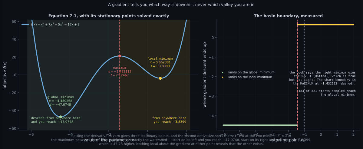
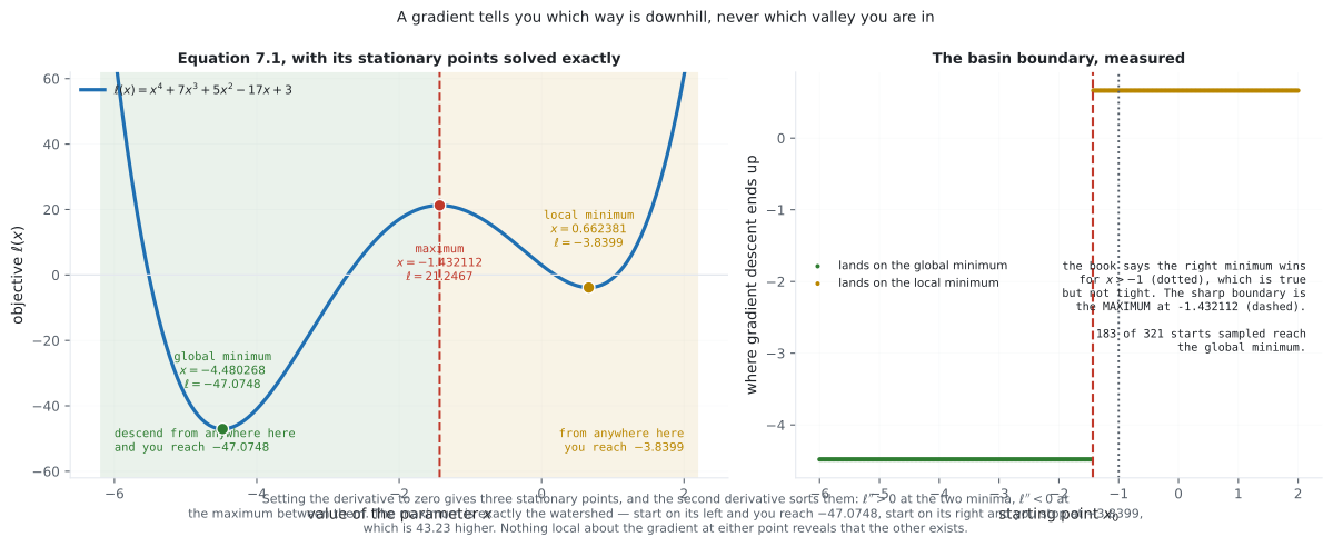
Reading the plot

The first figure separates two things the word “minimum” runs together. In the left panel the exact stationary points sit where the calculus puts them, and the shading is the measured basin of attraction: descend from anywhere green and you land on $-47.0748$; descend from anywhere amber and you stop at $-3.8399$, which is $43.23$ higher. The right panel makes the boundary explicit by running gradient descent from $321$ starting points and recording where each ends up. The split is perfectly clean and it falls at the maximum, $x = -1.432112$.

That is worth comparing against the book, which says the negative gradient leads to the right-hand minimum “for $x > -1$”. True — but conservative. The real watershed is $-1.432112$, so the interval $(-1.432, -1)$ is a strip the book gives away: start at $-1.4$ and you do reach the global minimum. Nothing hinges on it, but it is the kind of statement worth checking rather than absorbing, and the sharp version has a reason behind it: a watershed between two basins must be a stationary point, since the gradient has to change sign there.

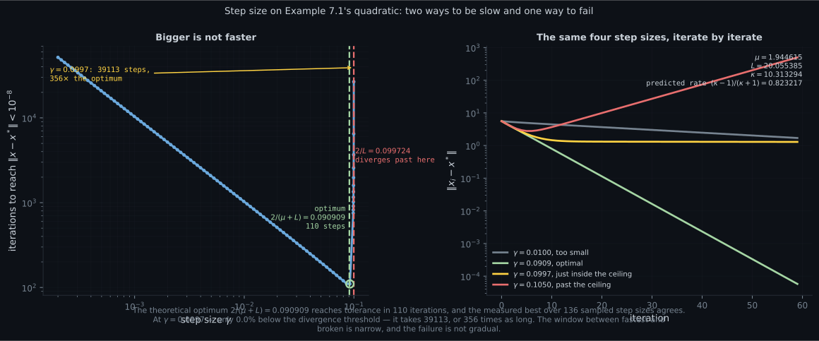
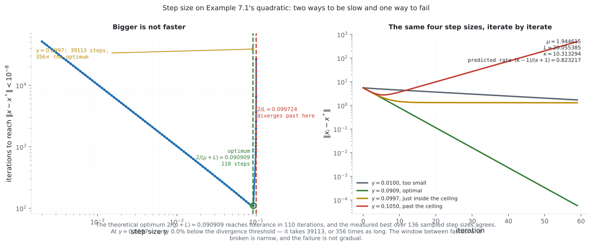
The second figure is the step-size story and its shape is the surprise. The instinct is that step size trades safety for speed monotonically — bigger is faster until it breaks. It is not. The curve is a U. Iteration count falls as $\gamma$ grows, bottoms out at $104$ iterations at $2/(\mu+L) = 0.090909$, and then climbs again, steeply, before the cliff at $2/L = 0.099724$. At $\gamma = 0.0997$ the method needs $39{,}113$ iterations. So the region just below the ceiling is almost as bad as a step size ten times too small, and it is the region a “keep increasing it while it still converges” search walks straight into.

The right panel shows why. Past the optimum the fast eigendirection is being overshot every step — its error factor $|1 - \gamma L|$ is heading back up toward $1$ from below — so it stops contracting while the slow direction is still crawling. Both modes must contract, and the binding constraint switches from the slow mode to the fast one exactly at $2/(\mu+L)$.

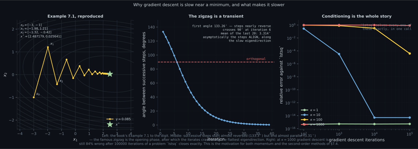
The third figure corrects a piece of received wisdom. Everyone learns that gradient descent zigzags in a valley, and the left panel shows it doing so. But the middle panel measures the angle between successive steps, and it decays: $133.26°$ between the first two steps (nearly a reversal), crossing $90°$ around the sixth, and averaging $3.31°$ over the last twenty. The steps end up almost parallel.

Both facts are real and they describe different phases. Early on, the error has a large component in the steep direction, that component is what the gradient mostly sees, and overshooting it flips the step — zigzag. That component dies quickly, at rate $|1 - \gamma L|$ per step. What survives is the error along the flattest direction, which contracts at only $|1 - \gamma\mu|$, and there the steps all point the same way. So the correct summary is: gradient descent zigzags briefly, then crawls. The crawl is the expensive part, and it is what momentum on the next page attacks.

The right panel prices conditioning. At $\kappa = 1$ the answer is exact after $100$ iterations. At $\kappa = 10$ it is exact by $10{,}000$. At $\kappa = 1000$, after one hundred thousand iterations the relative error is still $0.84$ — the method has barely started, on a problem lstsq closes exactly and instantly. That gap is the motivation for everything in §7.4: momentum, conjugate gradients, quasi-Newton methods, and preconditioning all exist to break the dependence on $\kappa$.

From the book

This page covers §7.1 and §7.1.1 of Mathematics for Machine Learning by Deisenroth, Faisal and Ong (draft of 2019-12-11). Equation 7.1 is the quartic objective, 7.2 and 7.3 its first two derivatives; Equation 7.4 is the minimisation problem, 7.5 the single step and 7.6 the gradient descent update. Example 7.1 is the two-dimensional quadratic with $\gamma = 0.085$ and iterates $[-1.98, 1.21]^\top$ and $[-1.32, -0.42]^\top$, illustrated in Figure 7.3. Equations 7.9 and 7.10 are Example 7.2, least squares by descent. The two adaptive step-size heuristics are attributed to Toussaint (2012); the condition number discussion and the preconditioner $\mathbf{P}$ follow Boyd and Vandenberghe (2004, chapter 9). Figure 7.2 is the plot of Equation 7.1 and Figure 7.1 is the chapter’s mind map. The Abel–Ruffini remark cites Abel (1826). The exact stationary points, the $2/L$ and $2/(\mu+L)$ formulas, the iteration counts and the conditioning sweep are this module’s additions.

Pitfalls

Reading a converged run as a global minimum

Gradient descent returns a point where the gradient is zero. Nothing about that point tells you whether a better one exists. In the opening example the two minima differ by $43.23$, and a run that started at $x_0 = 0$ reports $-3.8399$ with complete confidence. The only defences are knowing your function is convex (§7.3) or restarting from many initial points.

Assuming a bigger step size is faster right up to the cliff

Measured on Example 7.1: $\gamma = 0.0909$ takes $104$ iterations, $\gamma = 0.0997$ takes $39{,}113$. Both converge. The U-shape means a tuning loop that increases $\gamma$ while convergence still happens lands in the worst converging regime rather than the best one. Tune on iterations to tolerance, not on whether it converged.

Believing a run that is quietly diverging

At $\gamma = 0.09973$ — just $0.006\%$ past the ceiling — the error improves for the first $24$ iterations, reaching $1.332$, and then takes 30,262 more iterations to grow to ten times its starting value. A run that looks healthy for its first few hundred steps can be diverging. The reliable check is the growth factor $|1 - \gamma L|$, which is $1.000124$ here: greater than one, so the fast mode grows, so the run is doomed however good the first few steps look.

Forgetting the transpose in Equation 7.6

The book’s gradients are rows and the iterates are columns. In NumPy both are flat arrays, so the transpose is invisible and the code runs either way — which is precisely why the mistake survives into code that reshapes. The moment you introduce an explicit $(d, 1)$ column, x - gamma * grad silently broadcasts to a $(d, d)$ matrix. §0.2’s shape-checking habit catches it; NumPy does not.

Treating a stationary point as a minimum without checking the second derivative

$\nabla f = \mathbf{0}$ holds at minima, maxima and saddle points. In the opening example one of the three stationary points is a maximum; the saddle surface in the lab above stalls at a point that is a maximum in one direction. First-order information cannot tell these apart — that needs the Hessian, from §5.7.

Using gradient descent where a direct solver exists

Example 7.2 is a linear least-squares problem, and np.linalg.lstsq solves it exactly, in one call, at any condition number. At $\kappa = 200$ gradient descent was still $8.1\%$ wrong after $100{,}000$ iterations. Iterative methods earn their place when the problem is too large to factorise or has no closed form — not by default.

Compare

	gradient descent	Newton’s method (§5.7)	direct solve
information used	$f$, $\nabla f$	$f$, $\nabla f$, $\nabla^2 f$	the whole problem structure
cost per step	one gradient	a gradient, a Hessian, a linear solve	one factorisation
step size	must be chosen, $\gamma < 2/L$	none needed	not applicable
on a quadratic	$O(\kappa \log\frac{1}{\epsilon})$ steps	one step, exactly	exact
sensitive to $\kappa$	yes, severely	no	via numerical stability only
scales to millions of parameters	yes	no, the Hessian is $d \times d$	rarely

step size	behaviour on Example 7.1	iterations to $10^{-8}$
$0.0100$	safe, every step descends	$1025$
$0.0850$	the book’s choice	$112$
$0.0909$	$2/(\mu+L)$, provably fastest	$\mathbf{104}$
$0.0990$	past the optimum, fast mode overshooting	$1280$
$0.0997$	just inside the ceiling	$39113$
$0.0998$	past $2/L$	diverges
$0.1050$	well past	diverges

pch.quizTag Do you know what the step size can and cannot do?

1. Gradient descent converges and reports a point where the gradient is zero. What have you learned?

   A That the point is the global minimum of f B That the point is a stationary point, and without more information not even that it is a minimum C That f is convex D That the step size was chosen correctly
   pch.quizShowAnswer

   B — That the point is a stationary point, and without more information not even that it is a minimum — A zero gradient holds at minima, maxima and saddle points alike. Distinguishing them needs the second derivative, and ruling out a better minimum elsewhere needs either convexity or many restarts. In the chapter's opening example one of the three stationary points is a maximum and one of the two minima is 43.23 worse than the other.

2. On Example 7.1's quadratic, the fastest step size is 0.090909 and the divergence threshold is 0.099724. What happens at 0.0997?

   A It diverges, since it is essentially at the threshold B It converges in roughly 104 iterations, since it is below the threshold C It converges, but takes 39113 iterations — hundreds of times slower than the optimum D It converges faster than 0.090909, because the step is larger
   pch.quizShowAnswer

   C — It converges, but takes 39113 iterations — hundreds of times slower than the optimum — Iteration count against step size is a U, not a slide. Past 2/(mu+L) the fast eigendirection is overshot and stops contracting, so the count climbs steeply well before the cliff. Converging and converging usefully are different questions.

3. Why does gradient descent slow down as it approaches a minimum in a long thin valley?

   A The gradient magnitude shrinks, so the steps get shorter B The steep error component dies quickly, leaving the flattest direction, which contracts at only |1 - gamma*mu| per step C The step size automatically decreases near the optimum D Floating-point error dominates near the minimum
   pch.quizShowAnswer

   B — The steep error component dies quickly, leaving the flattest direction, which contracts at only |1 - gamma*mu| per step — Each eigendirection contracts by its own factor |1 - gamma*lambda|. The steep ones vanish fast, so what remains is the flattest, contracting at the rate set by the smallest eigenvalue. The measured angle between successive steps falls from 133 degrees to about 3 degrees, confirming the iterates end up crawling in one direction rather than zigzagging.

4. A run uses gamma = 0.09973 on Example 7.1, just past the 0.099724 ceiling. What does it look like?

   A It overflows within a few iterations B It improves for about 24 iterations, then takes tens of thousands more to visibly blow up C It converges, because the excess over the ceiling is negligible D It oscillates forever at a fixed distance from the minimum
   pch.quizShowAnswer

   B — It improves for about 24 iterations, then takes tens of thousands more to visibly blow up — The growth factor is |1 - gamma*L| = 1.000124: greater than one, so the fast mode grows, but only by 0.012 percent a step. Meanwhile the slow mode still contracts, so the total error falls at first. It took 30262 iterations after the turn to reach ten times the starting error. A healthy-looking first few hundred steps prove nothing.

5. What does the condition number kappa tell you about a gradient descent problem?

   A The largest safe step size B The ratio of the most curved direction to the least curved one, which sets how many iterations you need C Whether the objective has more than one minimum D Whether the gradient is a row or a column vector
   pch.quizShowAnswer

   B — The ratio of the most curved direction to the least curved one, which sets how many iterations you need — kappa is the ratio of largest to smallest singular value, and geometrically it is exactly the aspect ratio of the valley. The ceiling 2/L depends on L alone; the iteration count depends on the ratio. At kappa = 1000 gradient descent was still 84 percent wrong after 100000 iterations on a problem lstsq solves exactly.

🧪 Try It Yourself

Exercise 1 – Find and classify the stationary points

pch.exerciseTag pch.exerciseTitle

Exercise 2 – One gradient step, reproducing the book

pch.exerciseTag pch.exerciseTitle

Exercise 3 – The ceiling is 2/L and nothing else

pch.exerciseTag pch.exerciseTitle

Exercise 4 – Does f actually decrease every step?

pch.exerciseTag pch.exerciseTitle

Exercise 5 – Gradient descent against a direct solver

pch.exerciseTag pch.exerciseTitle

Recall card

• Equation 7.6 is the whole algorithm: x minus gamma times the gradient, transposed. Everything else in this chapter is a repair to it.
• The transpose is bookkeeping, not mathematics. Gradients are rows in this book, iterates are columns, and in NumPy the distinction is invisible until you reshape — at which point the subtraction silently broadcasts.
• Setting the derivative to zero is a definition, not a method. By Abel-Ruffini there is no general algebraic root for degree five or more, and a neural network’s stationarity condition is not even a polynomial.
• Example 7.1 exactly: A is [[2,1],[1,20]], b is [5,3], gamma is 0.085 from x0 = [-3,-1]. Then x1 = [-1.98, 1.21] and x2 = [-1.32, -0.42], and the exact minimiser is (97/39, 1/39) = [2.487179, 0.025641].
• Two numbers govern everything: mu = 1.944615 and L = 20.055385, so kappa = 10.313294. The ceiling is 2/L = 0.099724 and the fastest step is 2/(mu+L) = 0.090909.
• Iteration count against step size is a U, not a slide. 104 steps at the optimum, 39113 at 0.0997, divergence at 0.0998. Tune on iterations to tolerance, never on “did it converge”.
• A step past the ceiling can look healthy for a long time. At gamma = 0.09973 the error improves for 24 steps and needs 30262 more to grow tenfold. The reliable test is the growth factor |1 - gamma*L| against 1.
• The zigzag is a transient. The angle between successive steps falls from 133.26 degrees to a mean of 3.31 over the last twenty: gradient descent zigzags briefly, then crawls along the flattest eigendirection.
• The basin boundary is a stationary point. In Equation 7.1 it is the maximum at -1.432112, and the two minima differ by 43.23. The gradient never reveals which basin you are in.
• Conditioning, not step size, is the wall. At kappa = 1000 gradient descent is still 84 percent wrong after 100000 iterations of a problem lstsq closes exactly. Momentum, conjugate gradients and preconditioning all exist to break that dependence.
• Adaptive step sizes, two rules: if f went up the step was too large, so undo it and shrink gamma; if f went down, try a bigger one. The undo is what buys monotonic convergence.

Next: the first repair to Equation 7.6 — give it a memory. Momentum and Stochastic Gradient Descent