
The Maximum Variance Perspective
Page 1001 fixed the code length and left the basis open. §10.2 closes it, from one assumption:
If we interpret information content in the data as how “space filling” the dataset is, then we can describe the information contained in the data by looking at the spread of the data.
That is a modelling choice, not a theorem — and it is worth noticing that it is one, because §10.3 will minimise something apparently different and arrive at exactly the same .
What you’ll learn
Section titled “What you’ll learn”- Equations 10.7–10.9b: how “maximise the variance of the code” collapses to — one Chapter 6 identity and one line of algebra. Measured, all three readings agree to .
- Why the constraint is not cosmetic: without it the objective has no maximum at all.
- Equations 10.11–10.14: the Lagrangian, and the moment appears — “the Lagrange multiplier plays the role of the corresponding eigenvalue.”
- Equation 10.15, — measured for the first six components, largest gap . The variance you keep is the eigenvalue; there is nothing else to compute.
- Equation 10.17’s deflation and Equation 10.21’s claim that and share eigenvectors — verified by deflating four times and recovering each to under degrees.
- Equations 10.24 and 10.25: and , and the fact that the measured reconstruction error matches to — a result §10.3 will spend a whole section deriving.
- Why a random search is hopeless in dimensions: random unit vectors reach of , while power iteration reaches it in cheap steps.
Intuition: the objective is a function on a circle
Section titled “Intuition: the objective is a function on a circle”Strip §10.2 to two dimensions and the whole argument fits in one picture. A unit vector in the plane is just an angle. Feed it to and you get a number. Sweep the angle and you get a curve — and the curve has a maximum somewhere.
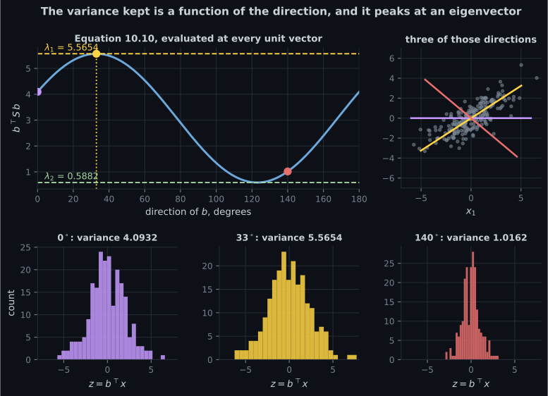
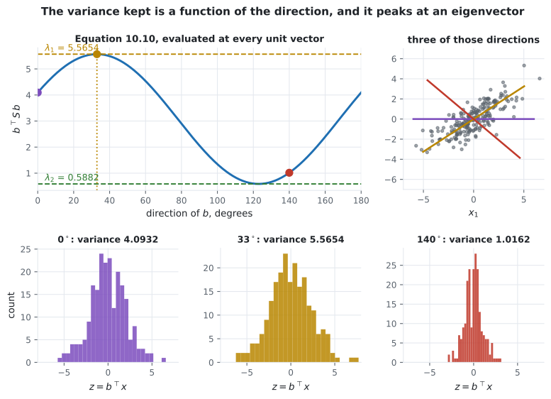
Two things the picture makes obvious that the algebra hides:
The curve is smooth and has exactly two stationary points on the half-circle — one maximum, one minimum. Those are the two eigenvectors. In dimensions there are of them, which is why one eigendecomposition answers the question for every at once.
You cannot find the peak by sampling. In two dimensions you could. In dimensions the surface of the unit sphere is overwhelmingly far from any particular direction: measured below, random unit vectors get to of the maximum.
§10.2.1 From “spread” to an eigenvalue problem
Section titled “§10.2.1 From “spread” to an eigenvalue problem”The variance of the first coordinate of the code, using the i.i.d. assumption:
Substituting and using the symmetry of the dot product, :
The only move is pulling outside the sum, which is legal because it does not depend on . Measured on the digit-”8” data, three routes to the same number:
| route | value |
|---|---|
| , Equation 10.7 | |
| , Equation 10.9b | |
np.var of the code | |
| , Equation 10.15 | |
| largest gap between any two |
(The code’s mean comes out at , so Equation 10.7’s “mean of the squares” really is the variance, as the book’s centred-data remark promises.)
The constraint is load-bearing
Section titled “The constraint is load-bearing”“Arbitrarily increasing the magnitude of the vector increases ” — doubling quadruples . So the unconstrained problem has a supremum of and no maximiser. Restricting to gives
and Chapter 7’s Lagrangian
Setting both to :
“By comparing this with the definition of an eigenvalue decomposition, we see that is an eigenvector of the data covariance matrix , and the Lagrange multiplier plays the role of the corresponding eigenvalue.” Measured — the gradient at three unit vectors:
| unit vector, with | gradient |
|---|---|
| a random direction (seed ) |
Equation 10.15, which is the whole point
Section titled “Equation 10.15, which is the whole point”Because and :
| gap | |||
|---|---|---|---|
The eigendecomposition does not just tell you where to look — it tells you what you will find there. No projection needs to be formed to know how much variance a component keeps. The book’s margin note adds the name: is the loading of , the standard deviation accounted for by .
§10.2.2 The second component, and why there is nothing new to do
Section titled “§10.2.2 The second component, and why there is nothing new to do”For with , the book’s device is to remove what the earlier components already explain:
then maximise against the deflated covariance, which is the §10.2.1 problem again. Run literally — deflate, re-decompose, take the top eigenvector, repeat:
| top eigenvalue of | of | angle to | |
|---|---|---|---|
| deg | |||
| deg | |||
| deg | |||
| deg | |||
| deg |
The book proves this must happen. Split the eigenvectors of by whether they have been used:
Expanding and applying each case gives
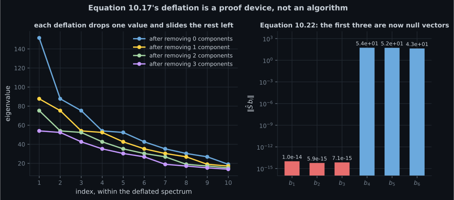
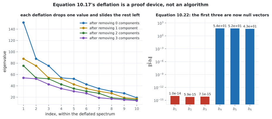
With Equation 10.21 in hand, for every (Equation 10.23), and summing:
Example 10.2, and the number the next section has to derive
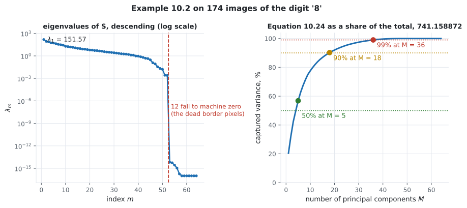
Section titled “Example 10.2, and the number the next section has to derive”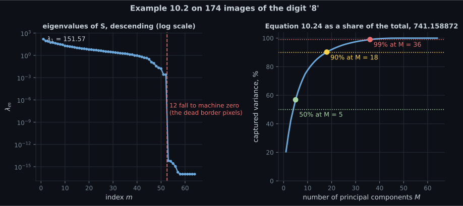
| (Eq 10.24) | (Eq 10.25) | share kept | measured | |
|---|---|---|---|---|
The last column was never mentioned in §10.2. It is the average squared reconstruction error, formed by actually building and measuring — and across every from to it agrees with to .
That equality is §10.3’s entire result, arrived at here for free. §10.2 maximised the variance kept; the error paid came out as the leftover eigenvalues without anyone asking. §10.3 turns the observation into a derivation, and Equation 10.44 will state it.
| variance retained | components needed | share of the dimensions |
|---|---|---|
-
Why does Equation 10.10 constrain b to have unit norm?
The book says it plainly: arbitrarily increasing the magnitude of b increases V1. The supremum of the unconstrained problem is infinity and no vector attains it. The constraint turns a meaningless problem into the one Chapter 7's Lagrangian solves, and the multiplier that appears turns out to be the eigenvalue.
pch.quizShowAnswer
B — Because without it the objective is unbounded — doubling b quadruples b-transpose S b, so there is no maximiser at all — The book says it plainly: arbitrarily increasing the magnitude of b increases V1. The supremum of the unconstrained problem is infinity and no vector attains it. The constraint turns a meaningless problem into the one Chapter 7's Lagrangian solves, and the multiplier that appears turns out to be the eigenvalue.
-
Equation 10.15 says V1 equals lambda-1. What is the practical consequence?
Measured for the first six components of the digit-8 covariance, b-transpose S b matches lambda to at worst 8.5e-14. One sorted list of eigenvalues prices every possible choice of M: V_M is the running sum and J_M is what is left, and the measured reconstruction error matches J_M to 2.8e-13.
pch.quizShowAnswer
B — The eigendecomposition already tells you the variance each component keeps — no projection needed — Measured for the first six components of the digit-8 covariance, b-transpose S b matches lambda to at worst 8.5e-14. One sorted list of eigenvalues prices every possible choice of M: V_M is the running sum and J_M is what is left, and the measured reconstruction error matches J_M to 2.8e-13.
-
What does Equation 10.21 establish about the deflated covariance S-hat?
Measured: deflating three times leaves S-hat b1, b2 and b3 with norms 1.0e-14, 5.9e-15 and 7.1e-15 — they are null vectors now — while the remaining eigenvalues match those of S to 7.8e-14. So the sequential search returns the eigenvectors of the ORIGINAL S, which one eigendecomposition already produced. Equation 10.17 is a proof device.
pch.quizShowAnswer
B — S and S-hat share eigenvectors; the used-up ones simply acquire eigenvalue zero — Measured: deflating three times leaves S-hat b1, b2 and b3 with norms 1.0e-14, 5.9e-15 and 7.1e-15 — they are null vectors now — while the remaining eigenvalues match those of S to 7.8e-14. So the sequential search returns the eigenvectors of the ORIGINAL S, which one eigendecomposition already produced. Equation 10.17 is a proof device.
-
Why is random search a bad way to find the direction of maximum variance?
Measured on the digit-8 covariance: the best of 200,000 random unit vectors scored 56.351776 against lambda-1 of 151.568412. Power iteration — repeatedly multiply by S and renormalise, Equation 10.52 — reaches the exact answer in 500 steps, landing 1.2e-06 degrees from b1.
pch.quizShowAnswer
B — In 64 dimensions the unit sphere is too large — 200,000 random unit vectors reached only 37.18 percent of lambda-1 — Measured on the digit-8 covariance: the best of 200,000 random unit vectors scored 56.351776 against lambda-1 of 151.568412. Power iteration — repeatedly multiply by S and renormalise, Equation 10.52 — reaches the exact answer in 500 steps, landing 1.2e-06 degrees from b1.
Exercises
Section titled “Exercises”Exercise 1 – Three ways to say the same variance
Section titled “Exercise 1 – Three ways to say the same variance”Exercise 2 – The Lagrangian’s gradient, and where it vanishes
Section titled “Exercise 2 – The Lagrangian’s gradient, and where it vanishes”Exercise 3 – Is lambda-1 really the maximum?
Section titled “Exercise 3 – Is lambda-1 really the maximum?”Exercise 4 – Deflate, and watch the eigenvalues not move
Section titled “Exercise 4 – Deflate, and watch the eigenvalues not move”Exercise 5 – Equation 10.25 predicts an error nobody measured yet
Section titled “Exercise 5 – Equation 10.25 predicts an error nobody measured yet”Recall card
Section titled “Recall card”- Section 10.2 assumes that information is spread, and derives PCA by maximising the variance of the code. That is a modelling choice, and Section 10.3 reaches the same answer from a different one.
- Equation 10.9b turns the objective into b-transpose S b in one line, using only the symmetry of the dot product. Measured three ways on the digit-8 data, all agreeing to 8.5e-14.
- The unit-norm constraint is load-bearing: doubling b quadruples the objective, so without it there is no maximum at all.
- The Lagrangian’s stationarity condition is the eigenvalue equation. Measured, the gradient is exactly zero at the leading eigenvector and 127.709219 at the second.
- Equation 10.15: the variance kept equals the eigenvalue. So one sorted eigenvalue list prices every possible choice of M, with no projection formed.
- Two hundred thousand random unit vectors in 64 dimensions reach 37.18 percent of the largest eigenvalue. Power iteration reaches it exactly in 500 steps.
- Equation 10.17’s deflation is a proof device, not an algorithm. S and the deflated S-hat share eigenvectors; the used-up ones simply acquire eigenvalue zero, measured at about 1e-14.
- So the greedy sequential choice is genuinely optimal, not merely locally optimal — the m-th round returns the m-th eigenvector of the original S.
- Equations 10.24 and 10.25 split the total variance into what is kept and what is lost, and the two always sum to the trace.
- The lost part equals the measured reconstruction error, to 2.8e-13, even though Section 10.2 never mentioned reconstruction. Section 10.3 derives that.
- On 174 images of the digit eight, half the variance costs 5 components and ninety-nine percent costs 36. Twelve eigenvalues are machine zero — the dead border pixels, free to discard.
Next: The Projection Perspective — the same , derived by minimising the reconstruction error instead, starting with the coordinates rather than the basis.
pch.coffeeTagline
pch.coffeeCtapch.feedbackHeading
pch.feedbackSubheading