
Capstone 2 - Churn with Point-in-Time Features
The decision
Section titled “The decision”A subscription business wants to spend a retention budget well. Every month, for each customer, it can send a retention offer or do nothing.
| Cost of an offer | EUR 4 to EUR 32, depending on what marketing chooses |
| Probability the offer retains a would-be churner | 0.30 |
| Value of a retained customer | EUR 120 |
| Churn rate | 41.75% of customers in the following month |
Contacting a customer is worth it when the expected saving exceeds the cost:
which is the same threshold derivation in a different costume. At an EUR 8 offer, contact anyone above 0.2222.
This capstone composes the point-in-time features, that threshold rule, and the honest-evaluation discipline from Phase 11.
Step 1 — the features could have existed
Section titled “Step 1 — the features could have existed”4,000 customers, 51,965 events in the 120 days before the cutoff, three features aggregated over the
final 30 days: event count, mean amount, and days since the last event. Every one computed by a function
that takes asof and never looks past it.
| Model | Test AUC | Test AP | Brier |
|---|---|---|---|
| point-in-time features | 0.7060 | 0.6010 | 0.2131 |
| the same window, ending 30 days later | 0.9564 | — | — |
The second row is the number this project exists to avoid. Moving the window to cover the month the
label describes gives +0.2504 of AUC, and every part of the pipeline still runs. The defence is that
window_features(events, 30, asof, ids) is called with asof = cutoff at training time and
asof = today at serving time — one function, one argument, and a
parity test
that proves the serving path agrees to floating-point tolerance.
Drawn on a timeline, the legal and illegal windows are one shift apart:
  flowchart LR
  subgraph HIST["days -120 to 0, before the cutoff"]
    E1["51,965 events"] --> W["feature window:
the final 30 days
count, mean amount,
days since last event"]
  end
  subgraph FUT["days 0 to +30, after the cutoff"]
    L["did the customer churn?
this is the label"]
  end
  W -->|"asof = cutoff"| M["model input"]
  L -->|"target"| M
  M --> OK["AUC 0.7060 -- honest,
and reproducible at
serving time"]
  E1 -.->|"window shifted 30 days later:
reads the same month
the label describes"| LEAK["AUC 0.9564 -- leakage.
Nothing errors. Every
test still passes."]
  LEAK -.->|"impossible in production:
those events have not
happened yet"| DEAD["the model that cannot
be served"]
The dotted path is the only difference between the two rows of that table: one argument to one function.
This is why asof is a parameter rather than an implicit “now” — a function that reads the clock cannot
be tested for point-in-time correctness, because there is no way to ask it what it would have known.
An AUC of 0.7060 is not impressive, and that is the point of the next step: the question is not whether 0.7060 is good, it is whether 0.7060 is worth anything.
Step 2 — price the campaign
Section titled “Step 2 — price the campaign”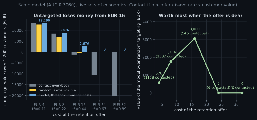
| Offer | Threshold | Contacted | Contact everybody | Random, same volume | Model | Model − random |
|---|---|---|---|---|---|---|
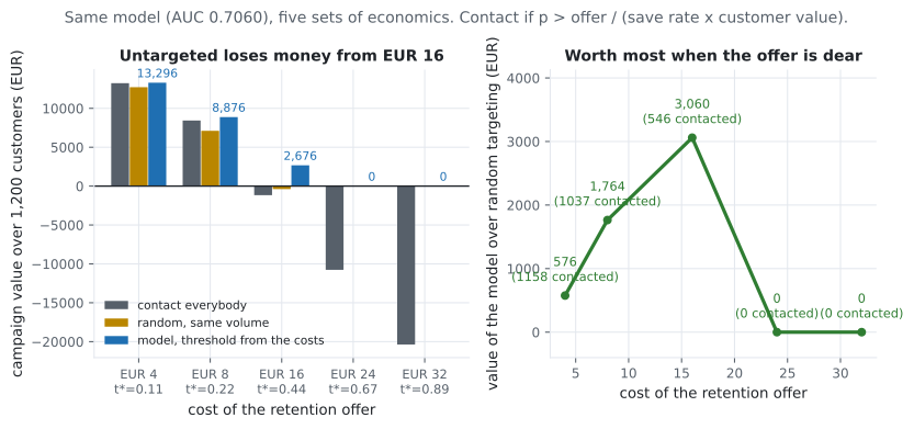
| EUR 4 | 0.1111 | 1,158 | EUR 13,236 | EUR 12,720 | EUR 13,296 | +576 |
| EUR 8 | 0.2222 | 1,037 | EUR 8,436 | EUR 7,112 | EUR 8,876 | +1,764 |
| EUR 16 | 0.4444 | 546 | −EUR 1,164 | −EUR 384 | EUR 2,676 | +3,060 |
| EUR 24 | 0.6667 | 0 | −EUR 10,764 | EUR 0 | EUR 0 | 0 |
| EUR 32 | 0.8889 | 0 | −EUR 20,364 | EUR 0 | EUR 0 | 0 |
Four conclusions, none of which are visible in an AUC.
A mediocre model can be very valuable — or worthless — depending on the economics. The same 0.7060 is worth EUR 576 at a cheap offer and EUR 3,060 at an expensive one. Report the value, not just the metric.
When the offer is cheap, do not build a model. At EUR 4, contacting everybody earns EUR 13,236 against the model’s EUR 13,296 — a 0.5% difference. The correct engineering decision is to send the offer to everyone and spend the modelling effort elsewhere.
The model’s value peaks where the decision is genuinely hard. At EUR 16 targeting is the difference between losing EUR 1,164 and making EUR 2,676. This is where a churn model earns its maintenance cost.
Above EUR 24 the honest answer is “no campaign”. The threshold 0.6667 exceeds every predicted probability the model produces, so it contacts nobody and returns exactly zero — which beats every alternative, including the untargeted campaign’s EUR 20,364 loss. A model that recommends inaction is doing its job.
See it move
Section titled “See it move”Three numbers set the whole policy: the offer cost, the save rate marketing promised, and what a customer is worth. The sketch puts all three on sliders and recomputes the threshold , the contacted set, and the campaign’s value — against contacting everybody and against no campaign at all.
Push the save-rate slider and watch what happens to “the model is worth”. At a 30% save rate and an EUR 16 offer the model earns its keep; drop the save rate to 15% and the threshold doubles to 0.8889, the campaign contacts nobody, and the model’s value becomes exactly zero — not because the model got worse but because the offer stopped working. The single most valuable experiment on this project is therefore a holdout group that measures the save rate, and it costs no data science at all. That is the finding worth taking to the campaign owner, and it is invisible in any model metric.
Step 3 — the numbers a campaign owner needs
Section titled “Step 3 — the numbers a campaign owner needs”CONFIG = {"offer_cost": 16.0, "save_rate": 0.30, "customer_value": 120.0}
def campaign(scores, config):
"""Everything the owner of the retention budget has to sign off."""
t = config["offer_cost"] / (config["save_rate"] * config["customer_value"])
contact = scores >= t
expected_saved = float((scores[contact] * config["save_rate"]
* config["customer_value"]).sum())
spend = float(contact.sum()) * config["offer_cost"]
return {
"threshold": round(t, 4),
"contacted": int(contact.sum()),
"share_of_base": round(float(contact.mean()), 4),
"spend": round(spend, 2),
"expected_value_saved": round(expected_saved, 2),
"expected_net": round(expected_saved - spend, 2),
"break_even_save_rate": round(config["offer_cost"]
/ (config["customer_value"]
* float(scores[contact].mean())), 4),
}break_even_save_rate is the field that survives contact with a sceptical stakeholder: it answers
“how effective does the offer have to be for this to pay for itself?” — and unlike the 0.30 assumption,
it is a number derived from the model’s own scores.
Step 4 — what to monitor, given the labels are 30 days late
Section titled “Step 4 — what to monitor, given the labels are 30 days late”Churn is only observable a month after the prediction, so nothing label-based is available on the day. What is available immediately:
| Signal | Why it matters | Where it comes from |
|---|---|---|
| contacted share (0.4550 at EUR 16) | budget consumption, today | the policy itself |
| mean predicted probability | drifts when the population or the pipeline changes | the scores |
| feature parity against the offline path | catches skew before performance moves | the parity test |
| schema violations per batch | a broken join changes features silently | the schema contract |
| realised save rate, when it arrives | the 0.30 assumption is the biggest lever in the model | the campaign’s own A/B test |
The last row deserves emphasis: the save rate is not a model parameter and nobody measured it. It came from marketing’s estimate, it appears in the threshold, and the whole business case is proportional to it. A holdout group that receives no offer is worth more than any modelling improvement on this page, because it turns 0.30 from an assumption into a measurement.
What this project does not solve
Section titled “What this project does not solve”- The offer’s effect is assumed, not estimated. Predicting who will churn is not the same as predicting who will be retained by an offer — that is uplift modelling, and it requires randomised holdouts to train on.
- A single cutoff. Real churn scoring runs monthly, so a customer appears many times; rows are not independent and a random split would leak across months.
- Censoring. Customers who churn after the 30-day window are labelled as staying, which biases the target towards imminent churn.
- The 41.75% base rate is unrealistic. Real monthly churn is a few percent, which makes the problem much more like the fraud capstone: average precision rather than AUC, and a threshold far from 0.5.
- Point-in-time features gave test AUC 0.7060, AP 0.6010, Brier 0.2131; the same window ending 30 days later reported 0.9564.
- Contact when — 0.2222 at an EUR 8 offer.
- At EUR 4 the model is worth EUR 576 over random and 0.5% over contacting everybody.
- At EUR 16 an untargeted campaign loses EUR 1,164; the targeted one earns EUR 2,676, and the model is worth EUR 3,060.
- Above EUR 24 the correct action is no campaign, and the model says so by contacting nobody.
- The campaign’s value is proportional to an unmeasured save rate of 0.30; a holdout group is worth more than any modelling change here.
-
Your churn model has AUC 0.7060. Is it good enough to deploy?
AUC is a property of the ranking; value is a property of the decision. At an EUR 4 offer, contacting everybody earns 99.5% of what the model earns, and the honest recommendation is to skip the model entirely.
pch.quizShowAnswer
B — The question is incomplete: the same model is worth EUR 576 at a cheap offer and EUR 3,060 at an expensive one, so value depends on the economics rather than the metric — AUC is a property of the ranking; value is a property of the decision. At an EUR 4 offer, contacting everybody earns 99.5% of what the model earns, and the honest recommendation is to skip the model entirely.
-
The retention offer costs EUR 16, and the untargeted campaign loses EUR 1,164. What does the model contribute?
This is where targeting earns its keep — the decision is genuinely hard, and the model's ranking is what separates the customers worth EUR 16 from the ones who are not.
pch.quizShowAnswer
B — It turns a loss into a profit: EUR 2,676 against minus EUR 1,164, and EUR 3,060 more than random targeting at the same volume — This is where targeting earns its keep — the decision is genuinely hard, and the model's ranking is what separates the customers worth EUR 16 from the ones who are not.
-
At an EUR 24 offer the model contacts nobody. Is that a failure?
A model that recommends inaction is doing its job. It also gives you a concrete improvement target: to keep the campaign viable at EUR 24 you need calibrated probabilities above 0.67, not a higher AUC.
pch.quizShowAnswer
B — No: t* = 0.6667 exceeds every probability the model produces, so no customer's expected saving covers the offer, and zero beats the untargeted campaign's EUR 10,764 loss — A model that recommends inaction is doing its job. It also gives you a concrete improvement target: to keep the campaign viable at EUR 24 you need calibrated probabilities above 0.67, not a higher AUC.
-
Which single investment would most improve this project's business case?
The save rate multiplies the entire value calculation and nobody measured it. It is also the gateway to uplift modelling — predicting who responds to the offer rather than who churns.
pch.quizShowAnswer
B — A randomised holdout that receives no offer, turning the assumed 0.30 save rate into a measurement — The save rate multiplies the entire value calculation and nobody measured it. It is also the gateway to uplift modelling — predicting who responds to the offer rather than who churns.
-
Why is a random train/test split wrong for a monthly churn scoring job?
The version on this page uses one cutoff and splits by customer, which is defensible. As soon as you score monthly, you need grouped, time-ordered splits — customers grouped, months ordered.
pch.quizShowAnswer
B — Because each customer appears at many cutoffs, so a random split puts the same customer's adjacent months on both sides and leaks — The version on this page uses one cutoff and splits by customer, which is defensible. As soon as you score monthly, you need grouped, time-ordered splits — customers grouped, months ordered.
🧪 Try It Yourself
Section titled “🧪 Try It Yourself”Exercise 1 – Build point-in-time features and the model
Section titled “Exercise 1 – Build point-in-time features and the model”Exercise 2 – Derive the contact threshold
Section titled “Exercise 2 – Derive the contact threshold”Exercise 3 – Price the model against two baselines
Section titled “Exercise 3 – Price the model against two baselines”Exercise 4 – Reproduce the leakage you are avoiding
Section titled “Exercise 4 – Reproduce the leakage you are avoiding”Exercise 5 – Report what the campaign owner signs off
Section titled “Exercise 5 – Report what the campaign owner signs off”Capstone 3 - Demand Forecasting for Ordering — from a contact decision to a quantity decision, where the asymmetry moves from the threshold into the loss function.
pch.coffeeTagline
pch.coffeeCtapch.feedbackHeading
pch.feedbackSubheading