LSTM & GRU Networks

The previous page left a SimpleRNN(32) at 0.5856 on IMDB — behind a bag-of-words model that has no concept of order at all. The problem is the recurrence itself: $h_t = \tanh(W_x x_t + W_h h_{t-1} + b)$ rewrites the entire state at every step, so information from step 5 has to survive 195 rewrites to reach the classifier.

Gated cells change one thing: the state is updated additively, under the control of learned gates, so information can be carried unchanged for as long as the gates say so. On the same data, same seed, same five epochs, that is worth +0.23 accuracy.

Cell	Total parameters	Recurrent layer only	Best validation accuracy	Seconds
`SimpleRNN(32)`	322,113	2,080	0.5856	29.5
`GRU(32)`	326,369	6,336	0.8156	52.3
`LSTM(32)`	328,353	8,320	0.8136	47.9

Most of those parameters are the 320,000-entry embedding matrix, identical in all three. The cells differ by 6,240 parameters and 0.23 accuracy.

What you’ll learn

The LSTM’s four gates and the GRU’s three, written out — and re-implemented in NumPy from a trained layer’s own weights, matching Keras to 6.56e-07.
Why a gate is exactly one more weight matrix pair: parameters scale 1 : 3 : 4.
What the gates actually did on a real review, including a forget gate averaging 0.7275 — a two-step half-life.
The one design decision that makes it work: the carry is scaled and added to, never overwritten.
Where GRU and LSTM differ, and how little it mattered on sentiment (0.0020) against how much it mattered at 80 steps (MAE 0.0056 and 0.0107 against a SimpleRNN’s 0.2984).
The same long-range experiment at a smaller budget, where every cell sat at the do-nothing baseline and would have supported the opposite conclusion.

The LSTM, exactly

Four gates, each a full linear layer over $x_t$ and $h_{t-1}$ :

\begin{aligned} i_t &= \sigma(W_i x_t + U_i h_{t-1} + b_i) && \text{input: how much of the candidate to write} \\ f_t &= \sigma(W_f x_t + U_f h_{t-1} + b_f) && \text{forget: how much of the carry to keep} \\ g_t &= \tanh(W_g x_t + U_g h_{t-1} + b_g) && \text{candidate: what could be written} \\ o_t &= \sigma(W_o x_t + U_o h_{t-1} + b_o) && \text{output: how much of the carry to expose} \end{aligned}

c_t = f_t \odot c_{t-1} + i_t \odot g_t, \qquad h_t = o_t \odot \tanh(c_t)

The second line is the whole idea. The carry is built by scaling the old value and adding — if $f_t \approx 1$ and $i_t \approx 0$ then $c_t = c_{t-1}$ exactly, and the information crosses the step untouched. A SimpleRNN cannot express that: every step pushes the entire state through a matrix multiply and a tanh.

The LSTM cell, from a trained layer's own weights

kernel, recurrent, bias = lstm_layer.get_weights()   # (features, 4U), (U, 4U), (4U,)
h = np.zeros(units, "float32")
c = np.zeros(units, "float32")
for x in sequence:
    z = x @ kernel + h @ recurrent + bias            # all four gates in one product
    i = sigmoid(z[:units])                           # Keras packs them i, f, g, o
    f = sigmoid(z[units:2 * units])
    g = np.tanh(z[2 * units:3 * units])
    o = sigmoid(z[3 * units:])
    c = f * c + i * g
    h = o * np.tanh(c)

Keras stores all four gates in one kernel of width $4U$ so four matrix multiplies become one — which is why the weight shapes look surprising until you know to slice them. Run this loop against the trained layer and the final prediction agrees to 6.56e-07 (0.414397 by hand against 0.414398 from Keras).

That equality is the point: the equations above are not a description of what TensorFlow does, they are what it does.

What the gates cost

Two panels. Left: parameters against units on log axes for three cells, with SimpleRNN lowest, GRU three times above it and LSTM four times above it, the three lines parallel. Right: a bar chart of weight-matrix pairs — 1 for SimpleRNN, 3 for GRU, 4 for LSTM — annotated with 2,080, 6,336 and 8,320 parameters at 32 units. — The ratio is exact and structural: every gate needs its own input matrix, its own recurrent matrix and its own bias. The parameter count still does not depend on sequence length — only on width and input size — so the cost of gates is paid once, not per timestep.

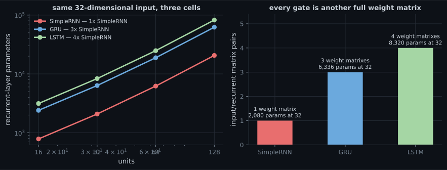
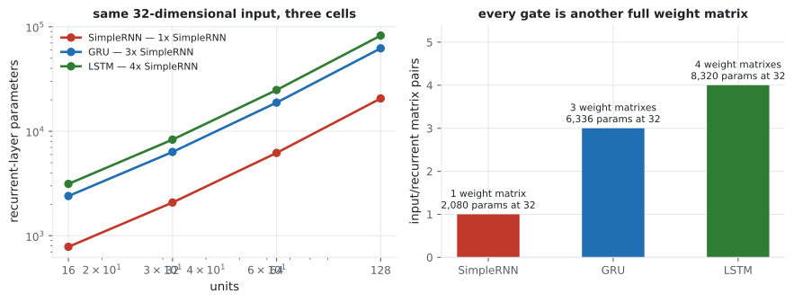
Units	`SimpleRNN`	`GRU`	`LSTM`
16	784	2,400	3,136
32	2,080	6,336	8,320
64	6,208	18,816	24,832
128	20,608	62,208	82,432

\text{params} = G \times \left(\text{features} \times U + U^2 + U\right), \qquad G = 1,\ 3,\ 4

Keras’ GRU carries a second bias vector for its reset-after variant, which is why 2,400 is a little above $3 \times 784 = 2{,}352$ .

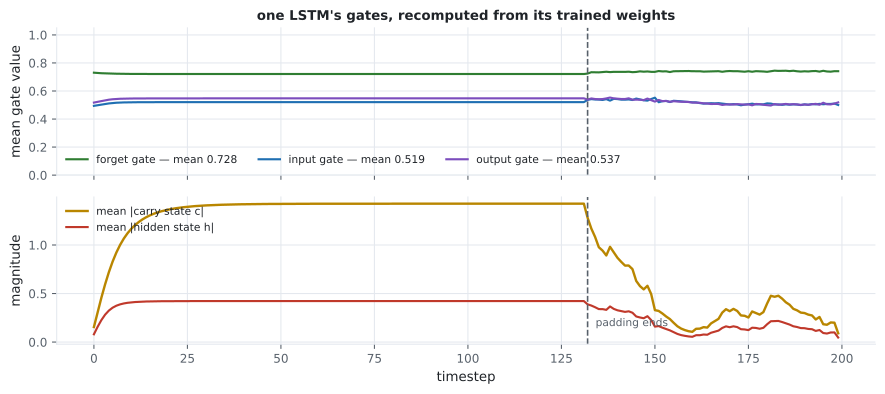
What the gates did

Take the trained LSTM(32) — validation accuracy 0.8136 — and recompute every gate for one review. This review is 68 tokens long inside a 200-step tensor, so it opens with 132 padding steps.

Two stacked panels sharing a timestep axis. The top shows three gate curves: forget flat near 0.73, input near 0.52 and output near 0.51 through the padding, becoming slightly noisy after step 132. The bottom shows mean absolute carry state rising to about 1.36 and holding flat, then falling sharply after step 132 towards 0.1, with the hidden state flat at 0.41 then falling to about 0.1. — Through the 132 padding steps every gate is constant — identical input, identical gates — and the carry settles at a mean magnitude of 1.3570. When the review begins at step 132 the carry collapses to 0.4186: the cell flushes the padding-induced state and starts storing the text instead. Note what the gates are not doing: they do not detect the padding boundary, they just respond to a different input.

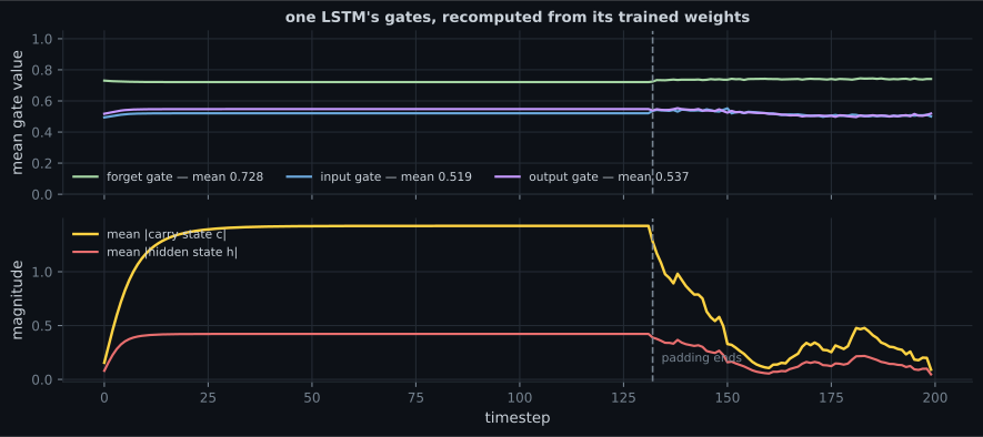
Signal	Mean over the padding	Mean over the text
forget gate	0.7215	0.7392
input gate	0.5199	0.5185
output gate	0.5467	0.5188
carry state \|c\|	1.3570	0.4186
hidden state \|h\|	0.4126	0.1786

Three honest observations:

The gates barely move between padding and text (forget 0.7215 → 0.7392). The states differ because the inputs differ, not because the cell recognised anything.
The carry is three times larger over the padding. Repeated identical input drives the additive update to a large fixed point that the first real tokens have to undo — the same attractor measured on the intro page, and a concrete reason to pass mask_zero=True.
A mean forget gate of 0.7275 is not long-term memory. $0.7275^{10} = 0.0412$ . This trained cell is smoothing over a few tokens, which is what sentiment needs. The capability to hold a value for hundreds of steps is there — it is what $f \approx 1$ means — but this task never asked for it.

The GRU: the same idea, one fewer gate

\begin{aligned} z_t &= \sigma(W_z x_t + U_z h_{t-1} + b_z) && \text{update: interpolate old and new} \\ r_t &= \sigma(W_r x_t + U_r h_{t-1} + b_r) && \text{reset: how much history the candidate sees} \\ \tilde{h}_t &= \tanh(W_h x_t + U_h (r_t \odot h_{t-1}) + b_h) \\ h_t &= (1 - z_t) \odot h_{t-1} + z_t \odot \tilde{h}_t \end{aligned}

	LSTM	GRU
states carried	two ( $h$ and $c$ )	one ( $h$ )
gates	4	3
parameters at 32 units	8,320	6,336
keep vs write	independent ( $f$ , $i$ )	coupled ( $z$ , $1-z$ )
measured here	0.8136 in 47.9s	0.8156 in 52.3s

The coupling is the real difference: a GRU cannot both keep the old value and write the new one, because its two weights sum to 1. An LSTM can. In exchange the GRU is 24% smaller, and here it scored 0.0020 higher — comfortably inside seed noise. Try both.

diagram Diagram mermaid

  flowchart LR
  subgraph simple["SimpleRNN: the state is overwritten"]
    A["h_{t-1}"] --> B["tanh(Wx·x + Wh·h + b)"] --> C["h_t"]
  end
  subgraph lstm["LSTM: the carry is scaled and added to"]
    D["c_{t-1}"] --> E["× f_t"] --> F["+ i_t ⊙ g_t"] --> G["c_t"]
    G --> H["h_t = o_t ⊙ tanh(c_t)"]
  end

Where all three still failed

The long-range test is the adding problem: uniform values with two marked positions — one near the start, one in the second half — and the target is the sum of the two marked values. Carrying a number the length of the sequence is the entire task, and predicting the mean sum of 1.0 is the do-nothing baseline.

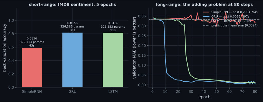
figure Short-range and long-range, the same three cells matplotlib

Two different arguments for gates. On IMDB (left) they are worth +0.23 accuracy for 3-4x the recurrent parameters. On the adding problem at 80 steps (right) they are worth the difference between working and not working at all: the GRU reached MAE 0.0056 and the LSTM 0.0107, while the SimpleRNN managed 0.2984 against a baseline of 0.3324 — a tenth of the way from doing nothing to solving it.

At 32 units and 80 epochs, the separation is total:

Cell	Recurrent parameters	Adding-problem MAE	Against the 0.3324 baseline
`SimpleRNN(32)`	1,153	0.2984	+0.0340
`GRU(32)`	3,489	0.0056	+0.3268
`LSTM(32)`	4,513	0.0107	+0.3217

The same experiment at a smaller budget said the opposite

The first version of this measurement used 16 units and 20 epochs:

Cell	Adding-problem MAE	Baseline
`SimpleRNN(16)`	0.3333	0.3324
`GRU(16)`	0.3005	0.3324
`LSTM(16)`	0.3328	0.3324

All three sat at “predict the mean”. Had the page stopped there it would have concluded that gates do not help with long-range dependency — the exact opposite of what the same code shows with four times the epochs. The adding problem is slow to crack, and a cell scoring at the baseline has not been shown to be incapable, only untrained. That failure is kept here on purpose, because it is the easiest way to publish a confidently wrong result.

sketch The carry state under a forget gate p5.js

Set the forget gate and watch how long one written memory survives. The trained LSTM's measured mean was 0.7275.

Drag the gate to 1.0 and the memory never decays. That is the regime the LSTM was designed for, and it is why Keras initialises the forget-gate bias to 1 by default (unit_forget_bias=True, Exercise 6): the cell starts out keeping its carry rather than erasing it.

sketch The measured table, ranked p5.js

Click a column to rank every row by it. The bars are that column's values and the highest and lowest are computed from the numbers, not written in.

Pitfalls

Assuming a gated cell fixes long range automatically. A measured 0.7275 forget gate is a two-step half-life. The capability exists; whether training uses it is up to the task.
Reading a baseline-level score as “this cell cannot do it”. At 16 units and 20 epochs all three cells sat at the adding-problem baseline; at 32 units and 80 epochs the GRU scored 0.0056. The first run measured the budget.
Choosing LSTM over GRU on principle. 0.8136 against 0.8156 here, with the GRU 24% smaller.
Slicing the gates in the wrong order. Keras packs one kernel of width $4U$ as i, f, g, o. Get it wrong and the cell runs silently and learns nothing sensible.
Ignoring what padding does to the carry. Mean |c| was 1.3570 over the padding against 0.4186 over the text — pass mask_zero=True.
Paying for gates on short sequences. At 10–20 timesteps a SimpleRNN is often fine and 3–4× cheaper.
Reporting a cell comparison without wall-clock. GRU and LSTM cost roughly 1.6× a SimpleRNN here, and on CPU that is the number that decides your iteration speed.

Recap

The LSTM’s four gates control an additive carry, $c_t = f_t c_{t-1} + i_t g_t$ — the mechanism a SimpleRNN lacks.
Keras packs the gates into one kernel of width $4U$ ordered i, f, g, o; the NumPy re-implementation matched Keras to 6.56e-07.
Parameters scale 1 : 3 : 4 — 2,080 / 6,336 / 8,320 at 32 units, independent of sequence length.
On IMDB: SimpleRNN 0.5856, GRU 0.8156, LSTM 0.8136. The gates were worth +0.23.
On the adding problem at 80 steps: GRU 0.0056, LSTM 0.0107, SimpleRNN 0.2984 against a 0.3324 baseline — and at a quarter of the budget, all three scored at that baseline.
Measured gate means: forget 0.7275, input 0.5192, output 0.5327; carry 1.3570 over padding against 0.4186 over the text.
GRU couples keep and write; LSTM keeps them independent. The two scored within 0.0020.

Dropout that actually works on a recurrent layer, stacking, and reading a sequence backwards: Advanced Recurrent Layers.

pch.quizTag pch.quizDefaultTitle

What does the LSTM have that a SimpleRNN does not?

pch.quizShowAnswer

B — An additive carry update, c_t = f_t·c_{t-1} + i_t·g_t — with f near 1 and i near 0 the carry crosses a step completely unchanged — A SimpleRNN pushes its entire state through a matrix multiply and a tanh at every step, so nothing can pass through untouched.
SimpleRNN, GRU and LSTM cost 2,080, 6,336 and 8,320 parameters at 32 units on the same input. Why that ratio?

pch.quizShowAnswer

B — Because each gate is another full weight matrix pair plus a bias — one set for SimpleRNN, three for GRU, four for LSTM — params = G*(features*U + U^2 + U) with G = 1, 3, 4. Keras' GRU adds a second bias vector, which is why it sits slightly above 3x.
The trained LSTM's forget gate averaged 0.7275. What does that imply about its memory?

pch.quizShowAnswer

B — An untouched memory decays about 27% per step — a two-step half-life, so this cell is smoothing over a few tokens rather than storing anything long-term — 0.7275^10 = 0.0412. The capability to hold a value exists (f near 1); this task simply never needed it.
On the adding problem at 16 units and 20 epochs, two of three cells scored at the do-nothing baseline. What follows?

pch.quizShowAnswer

B — Nothing about capability — the budget was too small, and a baseline-level score means untrained, not incapable — It is the same class of error as judging batch normalisation by a run too short for its moving averages to converge.
What is the practical difference between a GRU's update gate and an LSTM's input and forget gates?

pch.quizShowAnswer

B — The GRU couples them — it interpolates with z and 1-z, so it cannot keep the old value and write a new one at once; the LSTM's f and i are independent — That coupling is what saves the GRU a quarter of its parameters, and here it cost nothing measurable: 0.8156 against 0.8136.

🧪 Try It Yourself

pch.coffeeTagline

pch.coffeeCta

pch.feedbackHeading

pch.feedbackSubheading